Multiscale Gradient Correction

By Vicent Peris (PTeam/OAUV)
Published April 8, 2020

---

Introduction

One of the main goals of astrophotography is to show the natural scene in all of its purity, by removing instrument-related artifacts and any other light signals that don’t belong to the photographed object. This has only been possible since the beginning of the digital imaging era, because the linear response to light of image sensors allows us to correct all of these unwanted signal sources. Therefore, the digital sensor is the only means we have to reach an intimate meeting point with the natural object in our pictures.

Inside the image, there are signals that are external to the photographed object, such as the vignetting caused by the optical system, or the dark and bias patterns of the camera. We all know that we need to properly correct these instrumental signatures in order to generate a good master light. Other unwanted signals in the image are light gradients. Here we present a new observational method for correcting light gradients in astronomical images. This method has already been described briefly in my processing notes for the PuWe 1 image. Here we have an in-depth writing about the same technique. This gradient correction technique results from a careful analysis of the data present in my own pictures, and is working remarkably well in cases where software-based solutions cannot give reliable results.

Gradients and Information Reliability

During more than 20 years of imaging experience, I have seen very few cases of completely gradient-free images. In many cases, gradients are so intrusive that they have been the main depth-limiting factor in the image. In fact, you can shoot tens of hours of exposure time to record a faint and diffuse nebula but, if the resulting master light cannot be cleaned from intrusive light gradients, you won’t be able to show in a reliable way that nebula in the processed image. Gradient contamination alters local colors and brightness levels of low surface brightness nebulae. Even after applying gradient correction techniques, this contamination affects the image in a way that you cannot distinguish between gradient residuals and actual nebular features. In the case of the PuWe 1 image shown below, gradients cover the entire field of view.

It is important to understand that these gradients affect the image at a global scale, and that’s what makes correcting them so difficult. At a local environment, a gradient behaves as a constant shift in color and brightness. At a global scale, however, the problem is that we'd have to deal with different color and brightness biases that should be corrected locally in many different ways. It can be very complicated to achieve a homogeneous image, especially if we have low surface brightness, diffuse nebulae populating the background of the image. In the case shown above, there are many nebulae around the main subject that are equally important if we want to communicate the whole thing of the natural scene. We can give it a try with the DynamicBackgroundExtraction (DBE) tool, as shown on the mouseover comparison below.

The mouseover comparison with the original image shows that DBE, indeed, did a very good job. However, a careful visual inspection of the resulting correction shows subtle local variations in color and brightness that should make us doubt about the credibility of the image:

Now the question is: are those subtle color and brightness variations actual features of these objects? And the honest answer is: we don’t know. The reality is that we cannot perfectly correct gradients in our images, no matter which equipment or which technique we use. At a certain deepness in the image we’ll always start to guess whether a given structure is real or not. Of course, there is no problem if the full image is covered by bright nebulae; the problem arises when we try to image low surface brightness objects because there will be a higher probability of the gradients being stronger than those objects. The image shown above is a clear example of a DBE result not fulfilling our expectations, because at the level of the galactic cirrus we cannot discern the veracity of the remaining structures. This result imposes a serious limitation to the representation of the final picture, since we cannot show the galactic cirrus if we are not fully confident of the current information.

An Observational Gradient Correction Method

The proposed method uses observational data instead a purely software-based solution to remove the gradients in the image. The basic strategy is to tranform a global problem into a local problem.

This method uses an image acquired with a second telescope (T2) to derive the gradients present in the image of the first telescope (T1). The image of T2 should have a wider field of view than the one of T1:

There are two goals in this method. First, to simplify the gradients. Many gradients arise from optical properties of the imaging system. For instance, vignetting generates a radial gradient in the image. Below we present a synthetic radial gradient and its 3-dimensional representation.

At a local level, this gradient can be simplified to a linear gradient:

A 3-dimensional representation shows that this small crop can be approximated to a simple, linear gradient:

The second goal of this method is to simplify gradient correction by placing DBE samples outside of the field of view of T1, since the image of T2 has a wider field of view. This is very important for images where there are no real sky background areas in a narrow field of view.

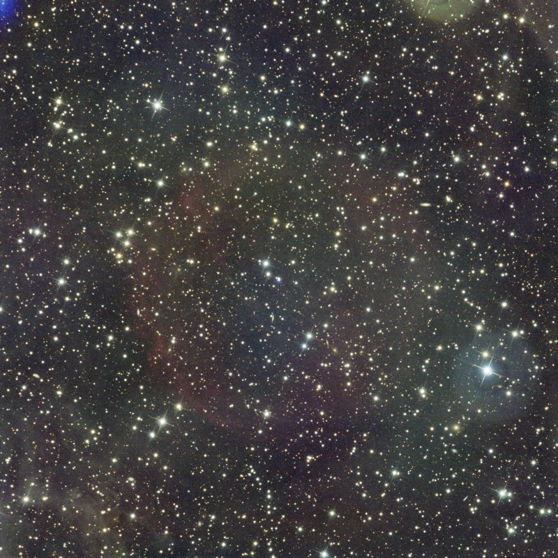
In the case of the PuWe 1 image, we have a second data set acquired with a Canon telephoto lens. The field of view of this lens is about 3×4 degrees, or about six times wider than the CDK20 image:

As any other image, this one has also its own suspicious gradients. This is easier to notice if we isolate the large-scale structures and enhance the contrast of the image:

It is impossible to know if those smooth color variations are real or not. But, what really matters, is that those gradients are almost negligible within the small field of view of the CDK20 image:

In this way the correction of gradients can be performed in a more reliable way, since we need to correct a field of view confined to a small area inside the T2 image. If we align the T2 image to the T1 image, we can see that the T2 image is much cleaner:

By using the T2 image as reference we can then subtract the gradients from the T1 image, even over extended objects.

This method requires an extra effort. For example, for this image, 22 hours of exposure through RGB filters acquired with the CDK20 telescope were corrected with 8 additional hours acquired with the Canon lens. In practice, this requires only a little more work for most astrophotographers. On one hand, most of us have a smaller OTA or a second camera; this is even more feasible today by using a cheap and sensitive CMOS camera. On the other hand, this extra exposure time can be acquired at the same time by placing the second OTA piggybacked on the main OTA.

This gradient correction method can deliver much more reliable results than an exclusively software-based solution:

In the next section we are going to describe the practical implementation of this method in PixInsight.

Multiscale Gradient Correction in PixInsight

Preparing the Images

We start with six master images: the R, G and B filters from both T1 and T2. These are the steps to follow:

• Compose both color images.
• If necessary, correct the gradients in the T2 image (the wide field one) with DBE.
• Apply a color calibration to both images.
• Align the T2 image to T1.

In the case of the PuWe 1 data, the wide field image is also contaminated with strong gradients:

It is obvious that we need to correct the gradients in the wide field image first, because this is our reference image for gradient correction in the narrow field image. We should then try to minimize the gradients in this image with the DynamicBackgroundExtraction tool:

It is important to keep in mind that no gradient correction can be perfect. What is important in this method is that the gradient correction applied to the narrow field image (T1) will be constrained by the local gradients in the wider field image (T2). Thus, even if we have some residual gradients in the T2 image, they will only cause a negligible effect in the T1 image.

Please note that we don’t touch the gradients in the T1 image at all. All of them will be corrected using the T2 image.

After this gradient removal, we calibrate the color of both images. We apply the PhotometricColorCalibration tool (PCC) using the same white reference for both images; in this case, we have used the average spiral galaxy white reference. Later we’ll see that this is an important step to simplify the gradient subtraction process.

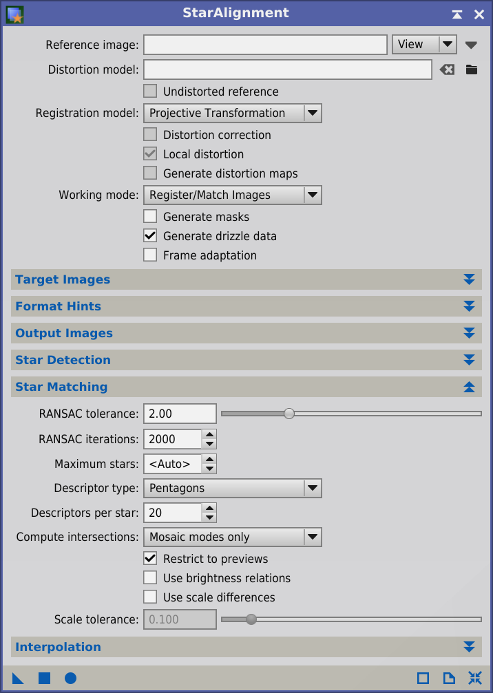
The last step is to align the T2 image to the T1 image. We use the StarAlignment tool with the T1 image selected as registration reference, since we need to align the wide field image, T2, to T1. This task can be delicate if there is a huge change of scale between both images. In cases where StarAlignment cannot find enough star pair matches as a result of too large scale differences, we can help the tool by creating a preview on the T2 image, roughly covering the field of the T1 image:

This preview points the tool to the area where star pair matches should be found. The option to restrict star matching to previews (Restrict to previews) is enabled by default (Star Matching section):

Generating the Gradient Model

The gradients will be calculated by comparing the T1 image to the aligned T2 image. This comparison will be done with PixelMath, but first we’ll duplicate the T1 image by dragging and dropping its main view selector to create a clone. We’ll rename this clone to “model”, since it will be the image that contains the gradient model after applying PixelMath to it. We have then three working images:

Since these gradients are always very smooth, we should compare only the large-scale structures of both images. We’ll isolate those structures with the MultiscaleMedianTransform tool (MMT), because the implemented nonlinear algorithm allows for a better isolation of small and bright structures over the nebulae, compared to other linear multiscale algorithms such as the Starlet transform. This can be done by disabling the first transform layers on the MMT tool:

These are the resulting images:

The gradients in the model image can then be extracted by subtracting the T2 image. This operation can be done with PixelMath. However, the formula cannot be as simple as "model – T2", because if we simply subtract one image from the other, we can easily clip the background as each image has its own background level. Therefore, when we subtract an image, we should also add its background level in the same equation. The correct PixelMath expression is hence:

model – T2 + med(T2)

In this PixelMath expression the med(T2) term represents the median pixel value of the T2 image, which is a good estimate of its background sky level. We should write this expression in PixelMath's RGB/K field:

This instance of PixelMath should be applied to the model image. With this operation we keep the sky background level of model unaltered after subtracting T2:

A careful inspection reveals that we are over-subtracting the nebula. In the mouseover comparison, it is noticeable because the red circle of the nebula is inverted after the process, generating a dark circle in the middle of the image. For an optimal subtraction, we should then scale the T2 image. This is implemented with the following PixelMath expression:

model – k*(T2 – med(T2))

where k is a scaling factor applied to the image without gradients. The key of this process is to manually find the optimal value of k by successive trials.

Remember that we previously applied PhotometricColorCalibration to both images. Since both images are referred to the same white point, now the k values for the three color channels should be very similar; in this case, a uniform value of 0.2 works very well:

Below you can see a mouse over comparison with different k values, from 0.1 to 0.3:

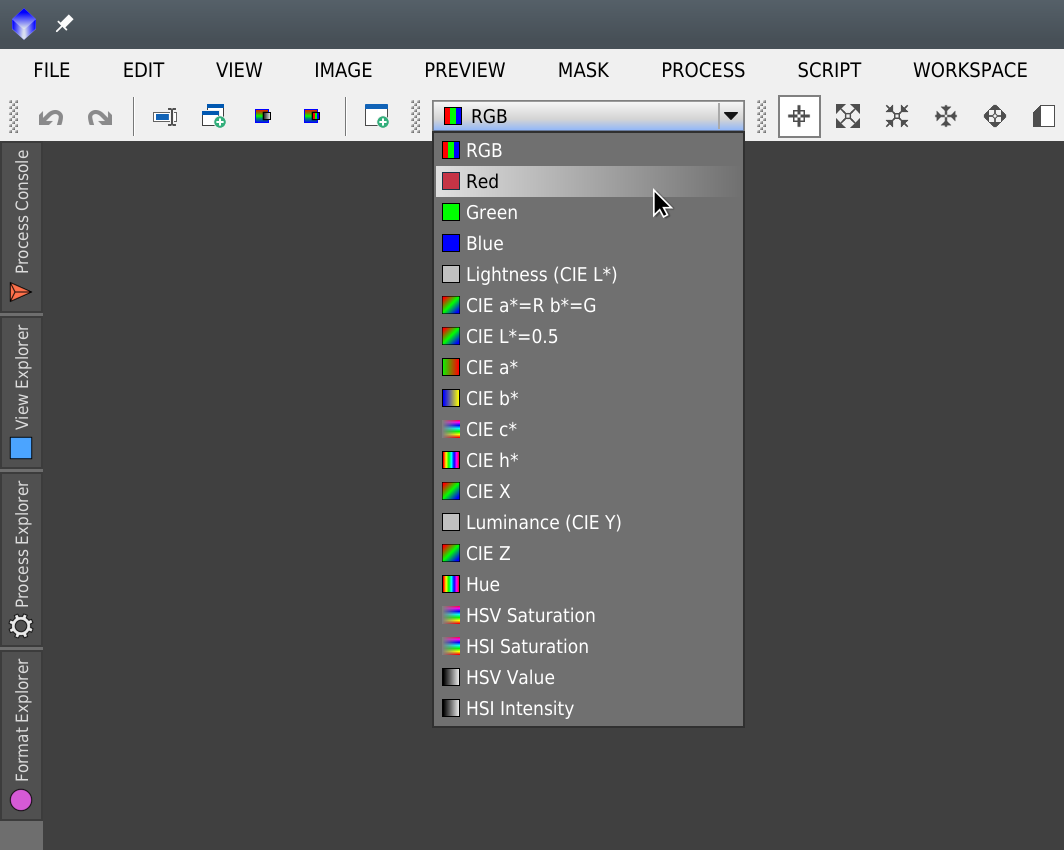
If required (mostly because white point calculation has its own associated error in each image), you can adjust this value separately for each channel by disabling the Use a single RGB/K expression option:

This is better done by visualizing each color channel with the Channel Selector while we adjust each k value:

Now let’s take a look at the model image after subtracting the T2 image with a scaling factor of 0.2:

By subtracting T2 we get the gradients in the model image. This result shows why a software-based solution will inevitably fail in all cases similar to this one: The gradients are fairly complex, but they also show complex structures that are completely embedded within the large nebula.

At this point there is still a question that remains unanswered: How many multiscale layers should we remove to generate the gradient model? On one hand, too few layers will leave traces of the stars and large-scale noise in the model. But, on the other hand, removing too many layers will soften too much the image, resulting in the lack of significant gradient structures. The mouse over comparison below shows the gradient models calculated by removing 6, 7, 8, 9 and 10 MMT layers.

You can see that by removing 8 layers we still have many residuals from stars. For this image we are removing 9 layers, but with the MultiscaleMedianTransform tool we cannot remove more than 8 layers. A workaround to this limitation is using the IntegerResample tool. First, we set the Resample factor parameter to 2 and check the Downsample option; then, the Downsample mode should be set to Median. The tool should be in the state shown below.

With these parameters the tool will use the median value of each block of 2×2 pixels to create a half-sized image. Now, in MultiscaleMedianTransform, the 8th layer will contain approximately the same structures as a hypothetical 9th layer at the original size of the image. If we'd set the Resample factor parameter to 4, then the 8th layer would contain the information of a 10th layer, and so on. In this case, since we need 9 layers, the workflow is to first apply IntegerResample to both images to decrease their sizes by a factor of 2, and then apply MultiscaleMedianTransform to them with the first eigth layers disabled.

Correcting the Gradients

Once we have the gradient model, we can subtract it from the T1 image with a similar PixelMath expression:

T1 - model + med(model)

Here we have the result:

Workflow Summary

The following figure is a workflow chart summarizing the methodology applied to the example described above.

Additional Examples

Abell 39

Abell 39 is a planetary nebula located in the Hercules constellation. The nebula is immerse in a dense field of background galaxies, but it also has a complex system of foreground, diffuse galactic cirrus. The data for this example have been acquired with the same instruments as the preceding one. We have a very deep image acquired with the Planewave CDK20 telescope, where the long focal length allows us to focus on the background galaxies. This image has gradients all over the diffuse cirrus. To correct them, we have used the Canon lens again. The total exposure times are 51 hours with the CDK20 telescope and 7 hours with the Canon lens.

This is the original CDK image:

And this is the Canon image, before and after gradient correction:

In the Canon image, we can see all the cirrus extending far beyond the field of view of the CDK20 telescope. Once we register the Canon image to the CDK20 image, we can see that there are significant data from these cirrus passing through the small field of view of the image:

Using the methodology described in this article, we can extract the gradients of the CDK20 image:

Once we have those gradients, we can subtract them from the CDK20 image:

A photometric analysis shows that, after the gradient correction, we reach very low surface brightness values. In the graph below, black corresponds to 30 mag/arcsec², and each step of gray represents an increment in brightness of 0.5 mag/arcsec².

It is also important to point out that the wide-field image is not just an auxiliary item to correct the narrow-field image. We can also have a wider, beautiful picture of the same object:

Click on the image to see a full-resolution version.

Barnard 63 and Jupiter

This technique can also be used in much wider field images. In this second example we show a picture of a conjunction between Barnard 63 and Jupiter, acquired with the 400 mm Canon lens. This picture shows a strong blue gradient towards the right side of the image because the first-quarter moon was 90° away from the object:

Located near the galactic plane, this is a dense stellar and nebular field. Here we have a good example of an image where we cannot apply software-based background modeling, since we probably don’t have a single pixel in the image corresponding to a free background sky area. Thus, it is completely impossible to generate a valid gradient model using DBE or any similar tool.

To subtract the blue gradient, we used a wide field image acquired with a Panasonic Lumix GX1 DSLR camera and a 25 mm f/1.4 lens. The wide field image, in this case, covers a big field of 29×38 degrees. Unfortunately, we have lost the original DSLR frames because of a hard drive failure, but we can show here the finished image:

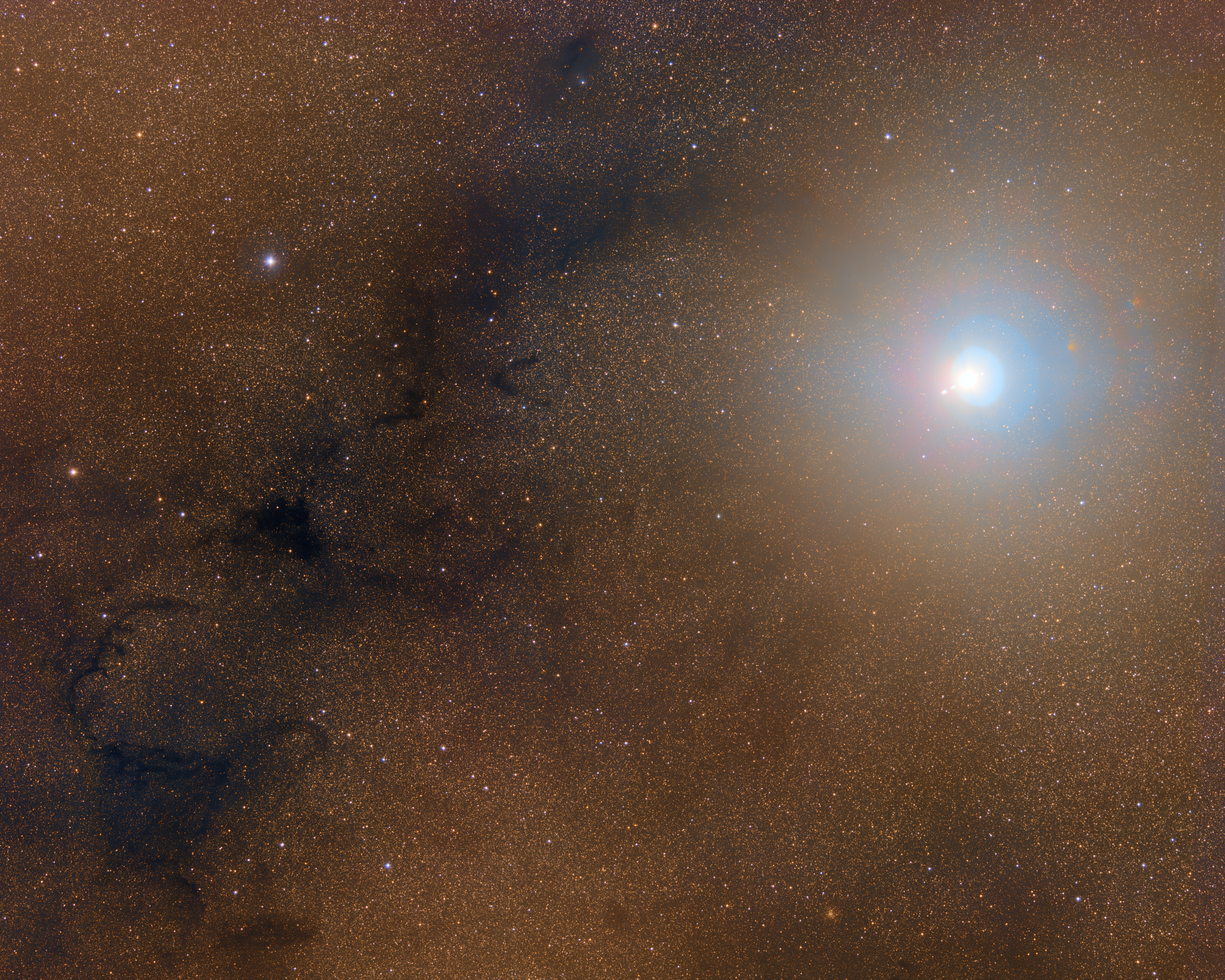
Click on the image to see a full-resolution version.

Conclusion

The last example with Barnard 63 and Jupiter shows that an efficient gradient correction can be performed even with small wide-field telescopes, simply by shooting ancillary images with a DSLR or a cheap CMOS camera coupled with a wide-field lens. In a future article we’ll write an in-depth review of this method applied to smaller-sized equipment, along with some new software tools that we are planning to implement, which will simplify and improve this technique.

The PuWe 1 and Abell 39 examples also show that gradient correction is an extremely delicate operation. Data reliability is always a critical problem in astrophotography because our picture is always based on the information that we can extract from the data. Our self-questioning in each of our works is crucial to achieve veracity in our images. Is that diffuse object in the image a real object? Or, is it just a defect coming from our own work? Would we want to enhance a feature that we really don’t rely on? We should consider that image processing is going to enhance some of the data in the image. Surely this will make our picture to appear deeper, but a superficial analysis of the data can lead to a completely wrong picture. This is particularly critical when we use multiscale techniques, since it is very easy to transform the artifacts in faint, background "nebulae".

On top of this discussion, there’s a more primary philosophical principle. This article shows that our creativity should always be ahead of the tools. We cannot expect a tool to satisfy all of our needs in all of our images, so we need to be creative, not only in our pictures, but also in the ways we use the tools available. PixInsight, and more specifically, PixelMath, are the tools that give us the freedom to be always at the forefront of the technique and artistic expression.