PuWe 1 Processing Notes
By Vicent Peris (PTeam/OAUV)
Published December 23, 2019
Introduction
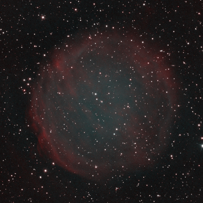
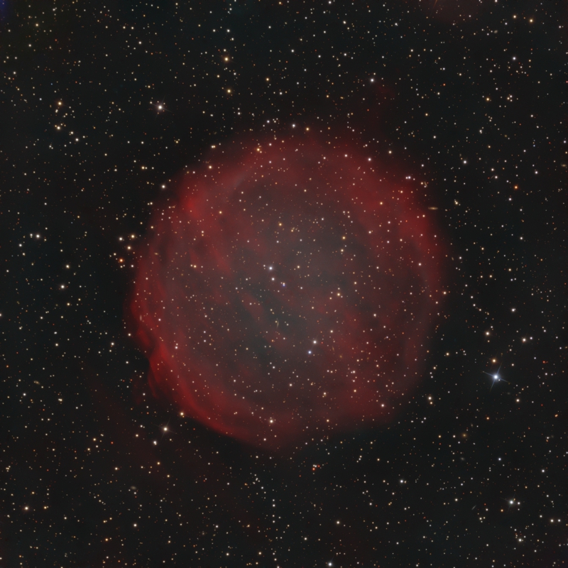
This article describes the processing performed for the PuWe 1 planetary nebula picture, which has been released on the official PixInsight Gallery. This text is not focused on describing particular processes or techniques, but on the building process of the image. This work integrates images acquired through six filters that describe very different aspects of the scene. While the H-alpha and O-III filters allow to image the extremely faint emission of this nebula, the wideband BVR filters capture star colors, foreground nebulae and background galaxies. Finally, the infrared filter highlights the infrared-emitting remote galaxies. All of these separate images should be merged into a single picture in a way resembling that the mixing process never existed. Therefore, tasks such as noise reduction acquire a new meaning because they are not applied with an aesthetic goal, but with a building goal, since they help to perform the mixing process smoothly. The text describes how we merge all of these components into the final processed picture.
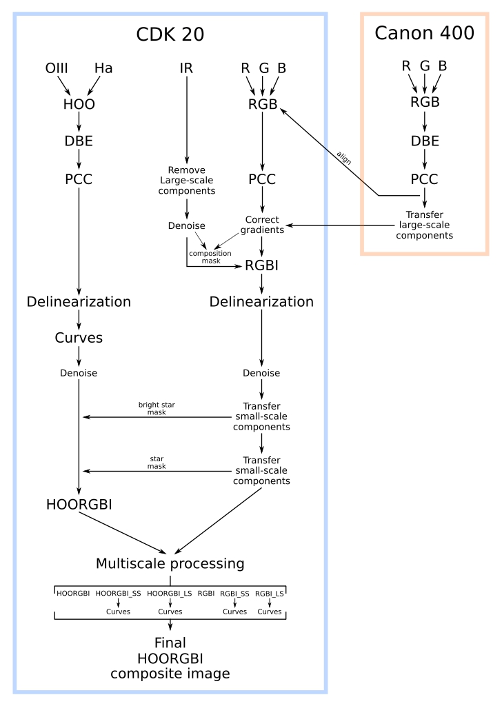
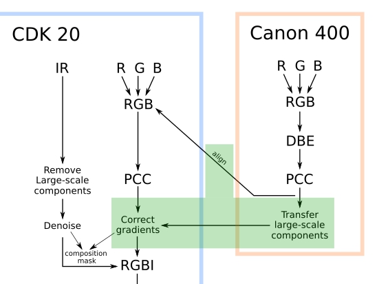
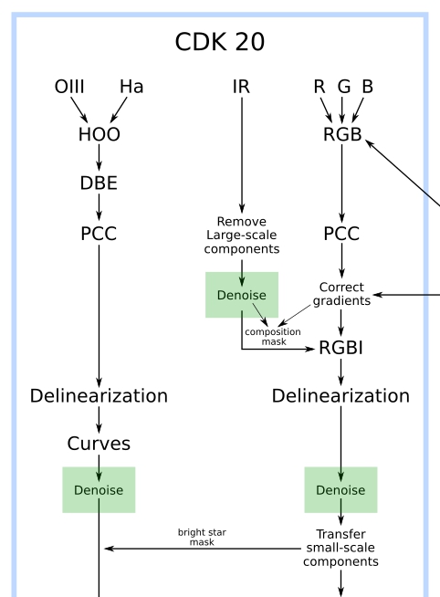
I’ve been working on this image for a total of ten months. This includes 120 hours of exposure time acquired during several months, as well as a big amount of time invested in the pre and postprocessing to have a final artwork that preserves both the beauty and the veracity of the scene. Many people I've been teaching during the last years asked me when I would start teaching advanced topics. This article is the first time I talk about an advanced workflow to summarize the entire postprocessing of one of my pictures, focusing on some steps and building blocks that I consider of special significance. I hope this article will offer you an inspiring point of view. The postprocessing workflow is schematized in the following figure.
The image presented here has been acquired with two different telescopes. Most of the data comes from a Planewave 20” CDK and a Finger Lakes Proline 16803. This data set comprises 4 broadband filters (Johnson B, V and R, and Sloan z’) and 2 narrowband filters (H-alpha and O-III), most of the exposure time (around 80 hours) coming from the narrowband filters. 8 hours of additional broadband data have been acquired with a Canon 400 f2.8 lens and a Finger Lakes Microline 16200 camera. The Canon lens data has been used to correct the gradients in the CDK image, as we'll see in the next section.
Most of the postprocessing work has been devoted to simplify the workflow to just the necessary processes. Every single step in the workflow above has its justification and every single detail has been thoroughly calculated.
This picture has also been a basis for the development of several new techniques and improvements in PixInsight:
- A new hardware-based gradient correction method, where the gradients are derived from the difference between wide-field and narrow-field images. We describe this method in this document.
- Two new scripts to detect and correct defective lines in subframes. The big improvement of these tools over other existing solutions is that we don’t paint the defects; instead, we calculate and correct the bias of these defects, preserving the original information in the image.
- A new narrowband working mode in the PhotometricColorCalibration tool to balance the emission line intensities in narrowband color images.
- A new method to integrate infrared data into RGB broadband color images, which we describe in this document.
This article is a write-up of some specific processes in the workflow. It does not describe all of the involved process in full detail, since it has been written to help understand the developments described above, and to give an architectural view of the picture, as well as to describe what’s inside my images, as this one is truly representative of my astrophotographic work.
Gradient Correction
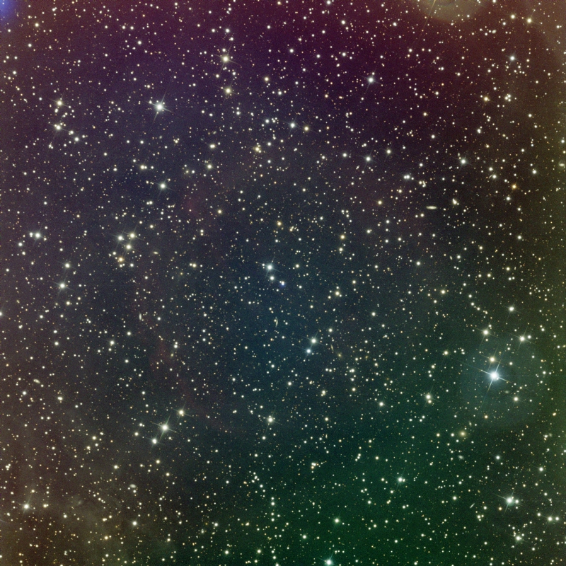
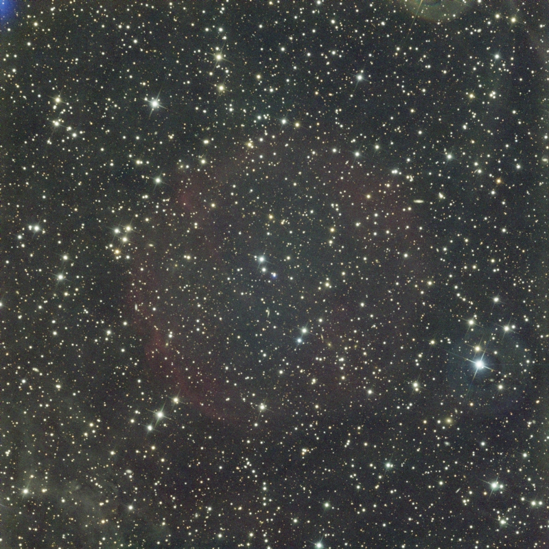
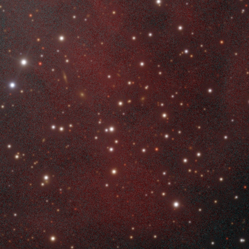
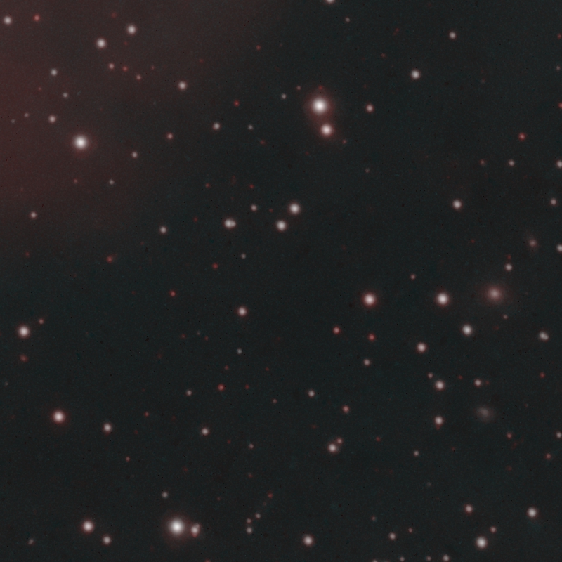
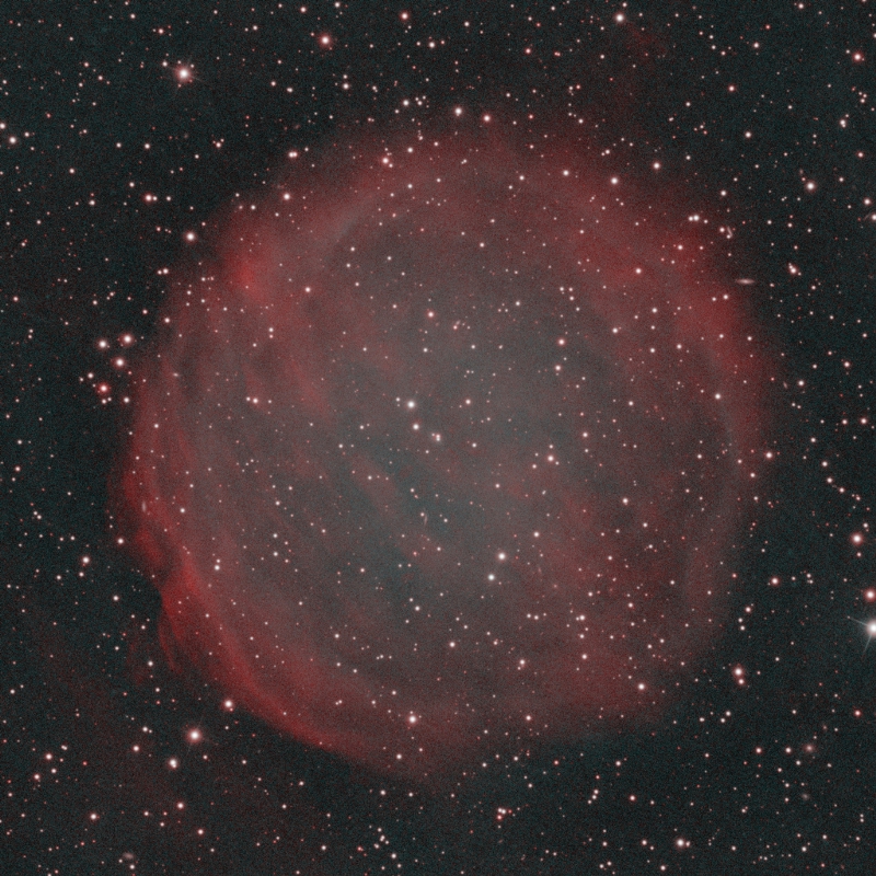
The RGB image acquired with the 20 inch telescope is affected by strong gradients that interfere with the low surface brightness background nebulae over the entire field in the image, as shown on the figure below.
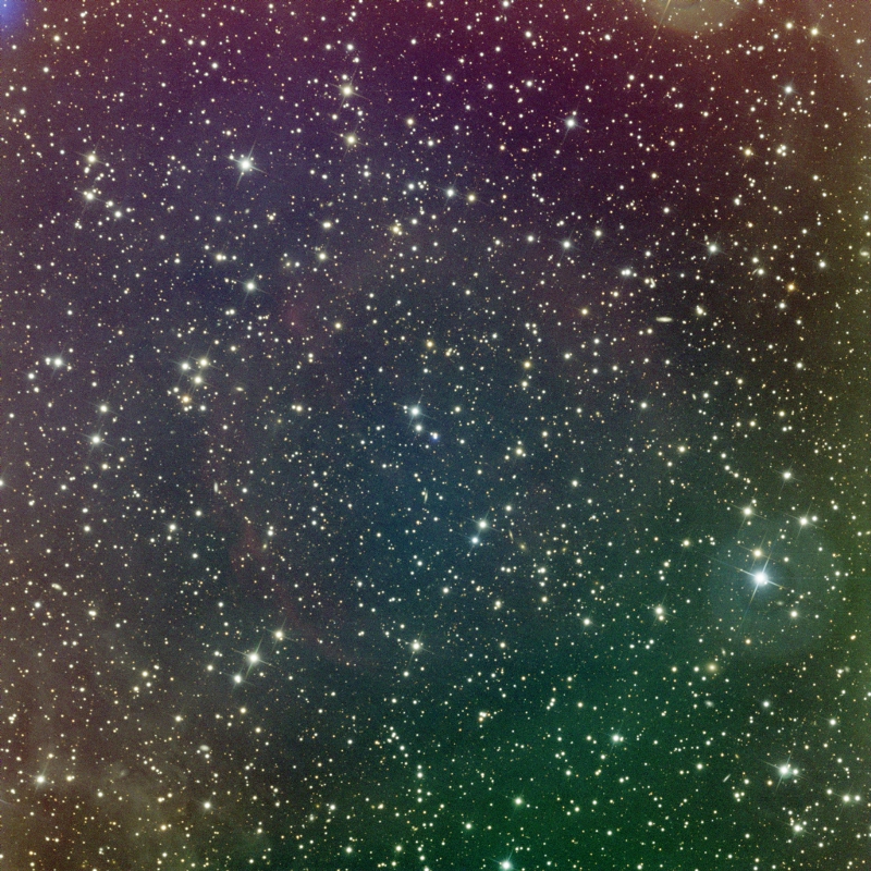
We can take care of these gradients with the DynamicBackgroundExtraction tool (DBE), which does a good job in a difficult scenario, as shown on the following comparison.
However, this image is a very difficult case where the entire field of view is covered by faint and diffuse galactic cirrus. They have an extremely low surface brightness and can be very easily contaminated by any stray light in the optics or any defect in the flatness of the flat field correction. This problem is especially remarkable when we try to do a color picture, since those artifacts can also easily colorize those nebulae. But the worst problem is that all of those artifacts are as faint and diffuse as the nebulae themselves.
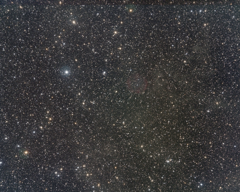
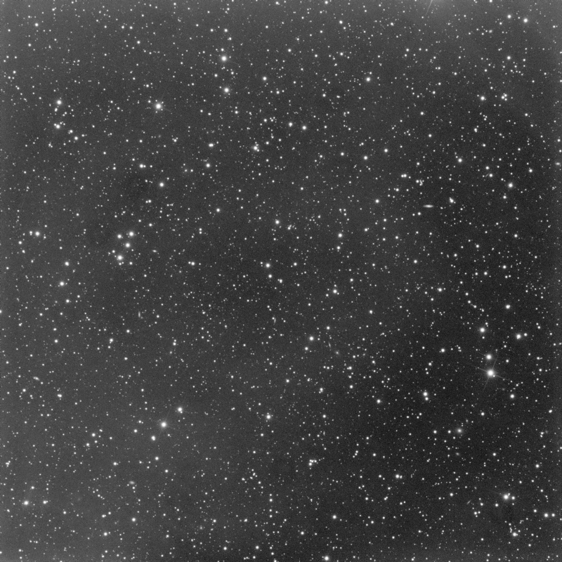
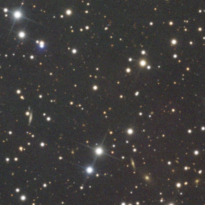
These nebulae are an important subject in the scene of this picture, so it is essential to be confident with the image and its content in these background areas. Here we present a new technique to correct gradients in the image with observational data, rather than using a software-based solution. The technique presented here uses a wide-field image to correct the gradients in the narrow-field image. You can see this wide-field image in the figure below.
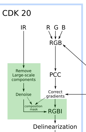
This gradient correction is applied after the color calibration of the 20 inch telescope image, as can be seen in the following workflow chart.
The idea behind this technique is that the residual gradients left in the image by optical reflections will be easier to correct in the wide-field image, since the field of view covered by the narrow-field image is only a small portion of the wide-field one. The next figure shows the regions of the sky covered by each image.
If we remove the stars in the wide-field image, we can see that there are also some residual gradients. However, since the narrow-field image covers a small portion of the wide-field image, the local residual gradients in the latter will be almost inexistent, as illustrated below.
Mouse over:
Canon 400 mm lens image.
Canon 400 mm lens image - large scales.
Canon 400 mm lens image - large scales - stretched.
Planewave 20" CDK image.
Therefore, if we correct the wide-field image at a local level, we can use it to flatten the narrow-field image.
Note that the yellowish/orange structure near the center of the image is actually a dust cloud, not an artificial gradient.
To apply the correction on the 20-inch telescope image we first align the wide-field image to the narrow-field one. In the comparison below you can see how well corrected is the wide-field image at a local level.
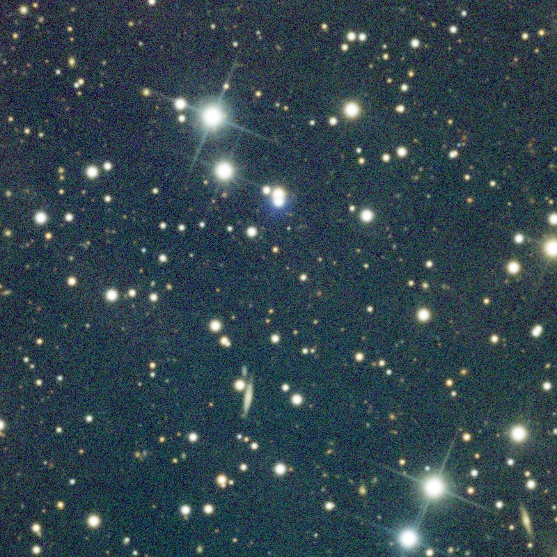
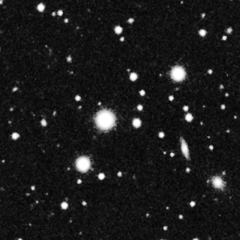
The resolution of the narrow-field image is obviously much higher:
The registered wide-field image shows interpolation ringing artifacts because we didn’t use drizzle to create the master lights, and those artifacts are magnified by the strong resampling applied by the image alignment process. Anyway, all of these problems are not relevant here since we are only interested in correcting smooth, large-scale gradients.
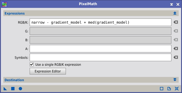
Those residual gradients can be extracted from the 20-inch telescope image if we subtract the wide-field image from it with PixelMath:

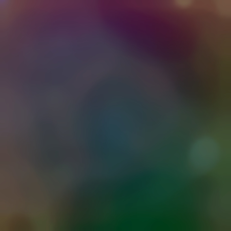
By subtracting the wide-field image, we obtain the residual gradients:
Mouse over:
20" CDK image.
Canon 400 mm lens image registered to CDK image.
Residual gradients in the CDK image.
The 0.2 factor in the applied PixelMath expression has been found manually by visual inspection of the resulting image. Too low of a value will leave traces of the nebula, and a value that is too high will start to invert it. The following comparison of results obtained with different factors will help understand this process.
Mouse over:
20" CDK image.
Subtract Canon lens image multiplied by 0.1.
Subtract Canon lens image multiplied by 0.2.
Subtract Canon lens image multiplied by 0.4.
We can avoid the artifacts around the stars and the noise in this gradient model by first removing the small scales of both images. This can be seen on the next comparison.
Mouse over:
Large-scale components of the CDK image.
Large-scale components of the Canon lens image.
Resulting residual gradients.
Now that we have a good gradient model, we can subtract it from the narrow-field image:
This operation results in a gradient-free image, which you can see on the following comparison.
In practice, these operations are equivalent to transferring the large-scale components of the wide-field image to the narrow-field image. However, by splitting the processes and inspecting the resulting models we can assure that the corrected image is free from residual artifacts.
With this technique we can achieve a much better correction than using software-based techniques, like DBE. Below we can compare the result with DBE to the result of this technique.
Mouse over:
20" CDK image.
20" CDK image corrected with DBE.
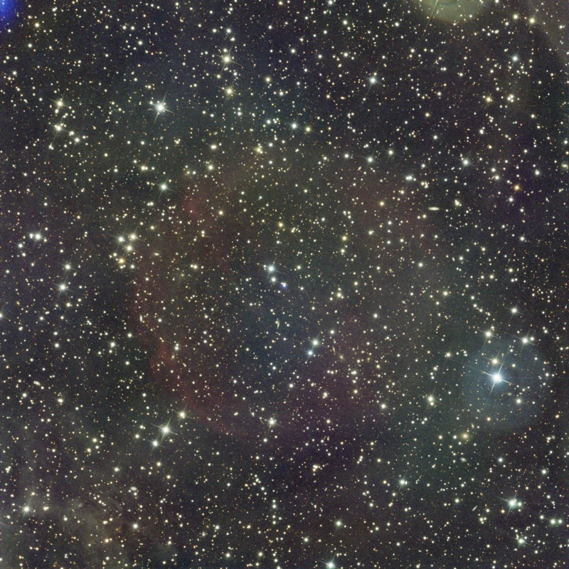
20" CDK image corrected with the Canon lens image.
By using the wide-field image as reference we are able to correct the gradients inside the large, diffuse nebulae, and we get a much better color uniformity over the entire image.
Image Composition and Noise Reduction
Multispectral images are difficult to compose because they require joining completely different images into a single color picture. Before attempting to integrate multiple channels in the color image, we should make them compatible. A critical aspect of this compatibility is the different noise level among the different images. We apply noise reduction to the individual components before the multiple composition processes in the workflow. We first denoise the infrared image before mixing it with the red channel of the broadband image. We also denoise the RGBI and the HOO images before performing the HOORGBI composition.
Below you can see a comparison of the mixing process between the red and the infrared images, with and without a prior noise reduction of the infrared image. Without noise reduction, the composition process leaves noisy areas around the infrared emitting objects.
Mouse over:
Infrared image added to the red channel without noise reduction.
Infrared image added to the red channel with noise reduction.
It is important to understand noise reduction as a process that allows us to merge all the components of the image, being essential to preserve the visual feeling of unity in the image throughout the creation process. This merging problem can be seen when we try to mix the HOO and RGBI images because the narrowband image is much noisier. Since we are placing the broadband objects over the narrowband image, the composition shows those objects surrounded by noiseless halos with the shape of the mask. Below you can see two crops showing the same processing workflow applied with and without these noise reduction steps in both images.

Integrating Infrared Data into Broadband RGB Images
Infrared Image Processing
An important subject of this picture is background galaxies. We use in this picture a Sloan z’ filter (which transmits the near infrared starting at 800 nm) to enhance the far and reddened galaxies. The quantum efficiency of the camera in this region of the spectrum is only an average of 15%, so the total exposure time of its image set is twice the exposures in the R and G filters.
In this section we describe how the infrared image is integrated into the broadband RGB image. This integration is applied to the RGB image after the gradient correction has been performed:
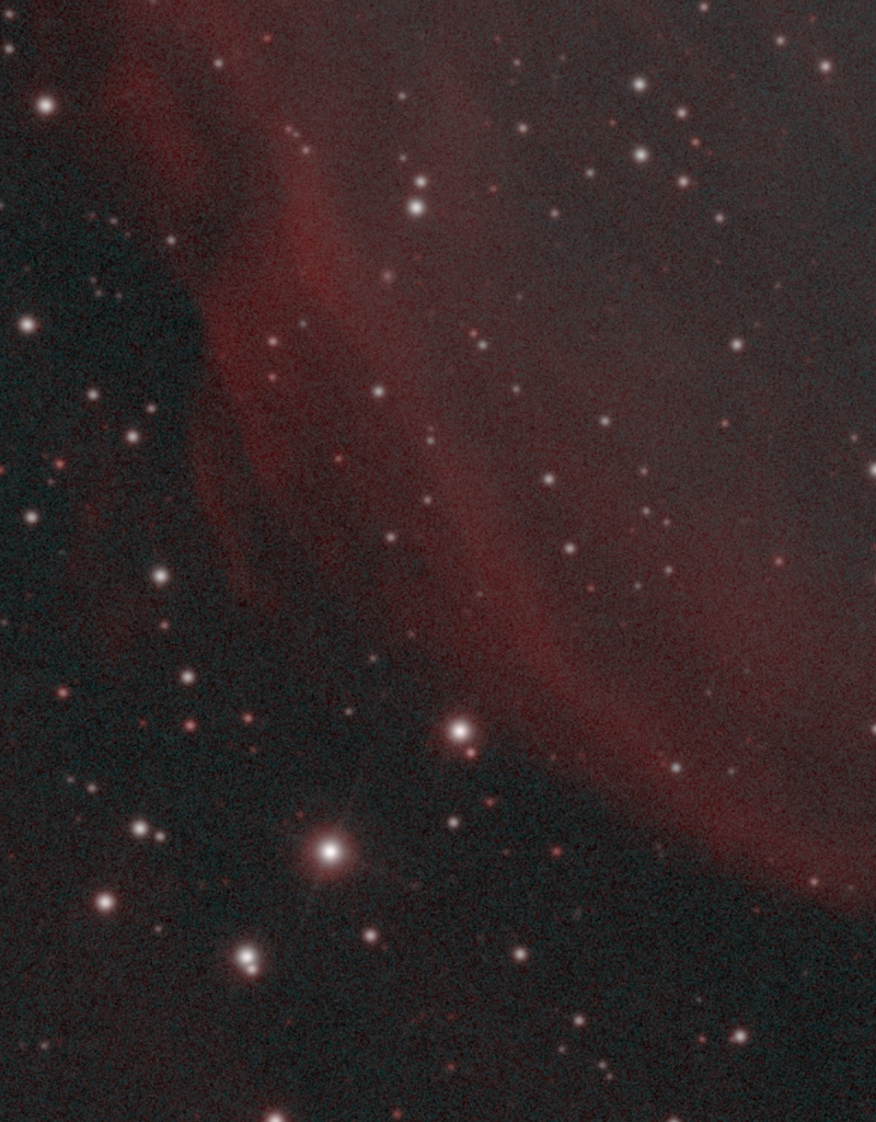
Before attempting the image combination, we need to optimize the infrared image. Anodized aluminum is very reflective in the near infrared, so it is very common to have strong gradients in an infrared image. Since we are only interested in small, point-like objects in the image, we simply remove the large scales, keeping only the structures in the scales from 1 to 64 pixels.
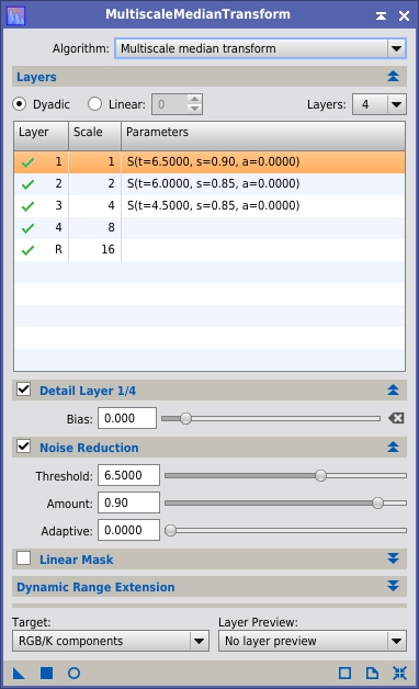
As noted previously, prior to combining both images we perform a noise reduction with MultiscaleMedianTransform (MMT) to the infrared image to ensure we don’t contaminate the color picture with noise:
This noise reduction is performed through a very restrictive mask that protects the small objects:
Below you can see the effect of the noise reduction process with MMT.

The denoised image still has large-scale noise over the background, but this won’t have any effect in the combined image thanks to the designed workflow, as I’ll explain later.
RGBI Composition
To proceed with the combination, we can add the infrared image to the red channel of the color picture using PixelMath.
In this PixelMath expression we add the infrared image, multiplied by 2, to the red channel. This means that we are enhancing the infrared emitting objects by a 200%. We also subtract the sky background level of the infrared image. In this way the sky background level of the color picture remains unaltered. You can see the resulting image below.
However, this simple operation does not provide an optimal result: Everything becomes very red in the picture, and only the very bluish stars remain with their original blue tones.
RGBI Composition Mask
We should now think on the goal of this process: To enhance the infrared emitting objects. Of course, almost every object in the picture emits in the infrared, but we want to highlight only those objects that have an excess in the infrared part of the spectrum. When we think about highlighting specific objects, that means we need a mask.
The objects that have an emission excess in the infrared are those that are brighter in the infrared than in the visible. If we select only those objects, we’ll be able to specifically enhance them in the color picture, leaving the rest of the objects with their original colors.
We can detect the infrared emitting objects with PixelMath using the following expression:
Let’s analyze this expression:
- We divide the infrared image by the maximum of the three color channels in the color picture. In this way any object in the picture that is brighter in the infrared than in the red, green or blue channels will have a value above 1.
- With the subexpression (z - med( z ) + med( rgb )) we assign the sky background level of the color picture to the infrared image. In this way both images will have the same sky background level. Since we are dividing the infrared image by the color image, the pixels over the sky background level will have a value of 1.
- The 1.1 factor establishes a clipping level. In the resulting image, the sky background will have a value of 1/1.1 = 0.91, and all objects having an infrared emission excess of more than 10% will be clipped to 1.
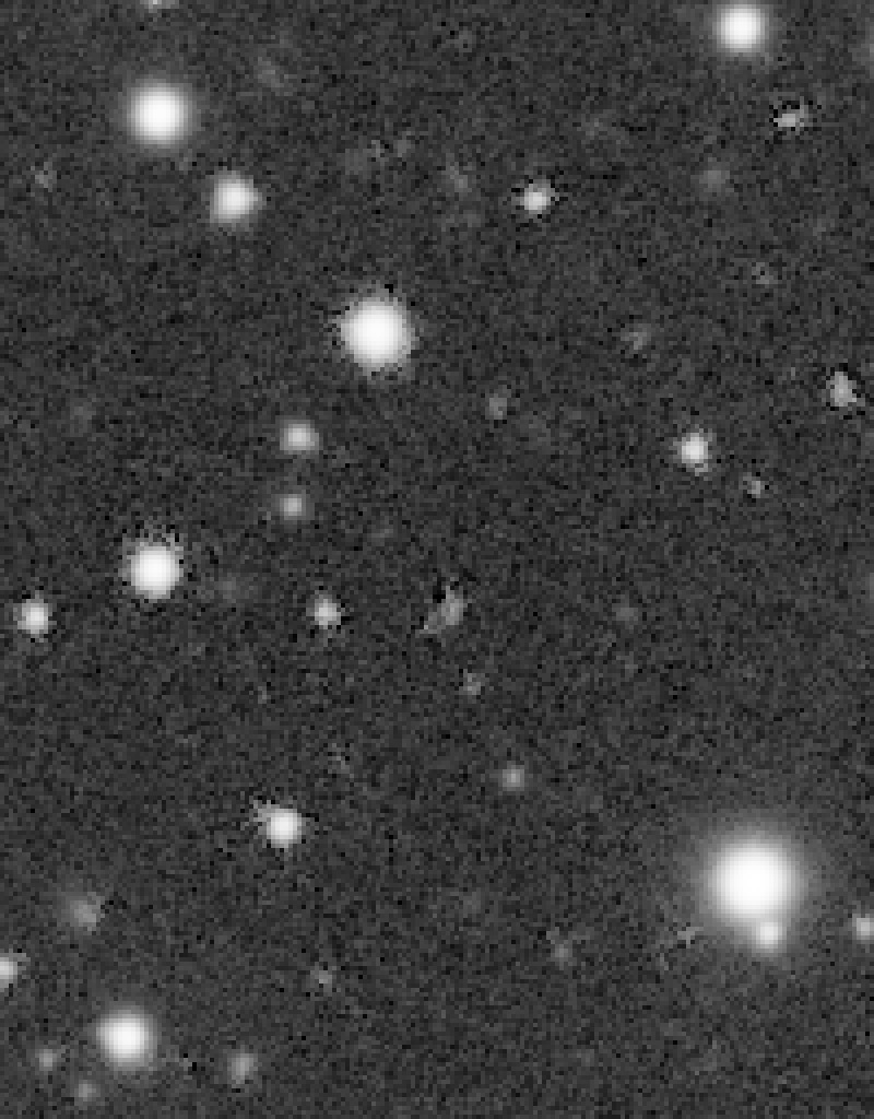
Let’s see the result on the following figure.

In this picture, the infrared emitting objects are clipped to white, the sky background is slightly darker, and the bluer objects are darker than the sky background. Since the infrared emitting objects are clipped, it is very easy to isolate them by using simple histogram transformations, as shown below.
Now that the objects we want to highlight are isolated by the mask, we can proceed again with the RGBI composition. Below you can see the result of the infrared enhancement through the mask.
Narrowband Image Composition
In this picture we assemble an HOO color image, where the H-alpha component goes to the red channel, and the OIII goes to both the green and blue channels, as shown below.

For this image, we developed the narrowband working mode in PhotometricColorCalibration. This option allows to calibrate the emission line intensities in a color image by rescaling each line. This way, the proportion between the different emission lines in the picture is the same as in the object in nature. Below you can see the result of color calibration.
Hexa-Band Image Composition
Composing the six bands together in a single color image has been especially difficult in this picture for one single reason: The gradient correction applied to the broadband image is so good that any slight color gradient in the narrowband image contaminates the color of the cirrus present in the broadband data.
We would usually mix all the six bands while the image is still linear. But this picture required to redesign the usual workflow and move the composition process to the non-linear stage of the workflow.

The logic here is simple: As we cannot apply the same gradient correction technique to the narrowband image, we are not completely sure of the veracity of the fainter areas in this image. Thus, to avoid affecting the fainter areas in the broadband image, we should control separately the contrast of these fainter structures in each image. The curves and the multiscale processing steps highlighted in the workflow allow us to control the contrast of the shadows independently in each image before performing the final hexa-band composition.
Recall that, before mixing both images, we apply a noise reduction to each one. This is particularly important in the narrowband image because the nebula is very noisy even with 80 hours of exposure time. The noise reduction of the narrowband image, as indicated in the workflow chart, is done after stretching the image, and it comprises three steps with MultiscaleMedianTransform. In the first noise reduction we work on the structures from 1 to 64 pixels. It is important to understand that many times you cannot perform a complete noise reduction in a single process, especially for difficult subjects like this nebula. In this picture, the second noise reduction provides an additional noise reduction over the fainter areas through a more restrictive mask to protect the inner nebula, as can be seen below.
Mouse over:
Narrowband image before second denoising process.
Narrowband image after second denoising process.
A third noise reduction is needed for the small scales after enhancing the overall contrast with histograms and curves. The following comparison shows the result of the noise reduction processes.
Below we show the MMT settings used for each of the three applied steps.
Mouse over:
Denoising process for the inner nebula.
Denoising process for the outer nebula.
Denoising process after contrast adjustment.
We use two different masks, the second being more restrictive for the inner nebula, since we focus the second noise reduction on the background. The masks are color images because in this way we improve protection of H-alpha structures, because the O-III image has a higher noise level. Below you can see both masks.
Keep in mind that these images are not the images being processed, but just the masks that we apply.
Once the HOO and the RGBI images have been delinearized, the overall contrast has been adjusted, and the noise reduction process has been applied, we perform the HOORGBI composition in three different steps.
The first two processes place the stars and galaxies over the narrowband image. This is done in two steps because we need to take special care of the bright stars. In the narrowband image, those stars show a differentiated halo coming from a reflection in the H-alpha filter. For this reason we need to replace the bright stars and their halos, which means that we need a star mask wide open to completely cover the halos. The second mixing process places the smaller stars and galaxies on the narrowband image, by using a star mask that selects all of them; in this second process we don’t need to open the mask since the halos don’t extend around the dimmer objects. We can see both masks below.

Below you can see the process to replace the stars and galaxies in the narrowband image on two selected areas.

Mouse over:
Narrowband HOO image.
Addition of bright stars and galaxies from broadband image.
Addition of dim stars and galaxies from broadband image.
Mouse over:
Narrowband HOO image.
Addition of bright stars and galaxies from broadband image.
Addition of dim stars and galaxies from broadband image.
Multiscale Processing
The result above transfers the small objects from the broadband image to the narrowband image, but this composition lacks the low surface brightness of the cirrus in the broadband image.
To enhance these nebulae in the final composed image, we split the large-scale and small-scale components of the HOORGBI image that we built above and the ones from the RGBI image. Then we have six images that we’ll process separately:
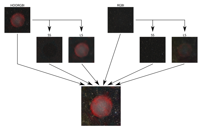
These six images can be recombined with PixelMath, with their proper weights to produce a final version with enhanced cirrus:
The multiscale splitting workflow allows to have a picture we can be confident of, since we separately control each component of the image and balance it with the rest.
Processing Summary
The comparison below summarizes the postprocessing of this picture.