
Hi all,
The latest version 1.6.1 of PixInsight comes with a couple new features implemented in the ImageIntegration tool. This is a brief description of both, where I'll borrow some figures and text from other posts to make up a sort of official description.
Linear Fit Clipping Pixel Rejection Algorithm
The new Linear Fit Clipping rejection method fits the best possible straight line, in the twofold sense of minimizing average deviation and maximizing inliers, to the set of pixel values in each pixel stack. At the same time, all pixels that don't agree with the fitted line (to within user-defined tolerances) are considered as outliers and thus rejected to enter the final integrated image.
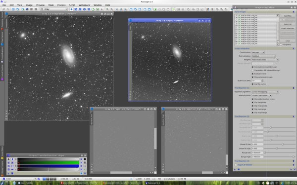
The new pixel rejection algorithm is controlled, as usual, with two dedicated threshold parameters in sigma units: Linear fit low and Linear fit high, respectively for low and high pixels. The screenshot below shows the new version of ImageIntegration and some results of the new rejection method.
The difference between linear fit clipping and sigma clipping is best explained with a graphical example. Consider the following figure.
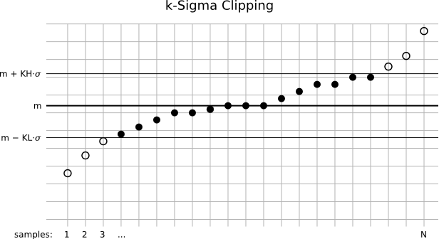
Suppose we are integrating N images. In the figure, we have represented a stack of N pixels at the same coordinates, whose values have been sorted in ascending order and plotted as circles on the graphic. The horizontal axis is the ordered sample number, and the vertical axis represents the available range of pixel values.
What we pursue with pixel rejection is to exclude those pixels that have spurious values, such as pixels pertaining to cosmic rays, plane and satellite trails, and other too high or too low pixels that are not valid data for some reason. We want to reject those pixels to make sure that they won't enter the integrated image.
The symbol m represents the median of the distribution. The median is the value of the central element in the ordered sequence, which in statistical terms corresponds to the most probable value in the distribution. Here, the median is being used as a robust estimate of the true value of the pixel, or more realistically, the most representative value of the pixel that we have available. Robustness here means unaffected by outliers. An outlier is a value abnormally low or high, as are both extreme values in the graphic, for example. Outliers are precisely those values that we want to exclude, or reject. By contrast, valid pixel values or inliers are those that we want to keep and integrate as a single image to achieve a better signal-to-noise ratio. Our goal is to reject only really spurious pixels. We need a very accurate method able to distinguish between valid and not valid data in a smart way, adapted to the variety of problems that we have in our images. Ideally no valid data should be rejected at all.
With two horizontal lines we have represented the clipping points for high and low pixels, which are the pixels above and below the median of the stack, respectively. Pixels that fall outside the range defined by both clipping points are considered as outliers, and hence rejected. In the sigma clipping algorithm, as well as in its Winsorized variant, clipping points are defined by two multipliers in sigma units, namely KH and KL in the figure. Sigma is an estimate of the dispersion in the distribution of pixel values. In the standard sigma clipping algorithms, sigma is taken as the standard deviation of the pixel stack. These algorithms are iterative: the clipping process is repeated until no more pixels can be rejected.
In the figure, rejected pixels have been represented as void circles. Six pixels have been rejected, three at each end of the distribution. The question is, are these pixels really outliers? The answer is most likely yes, under normal conditions. Normal conditions include that the N images have flat illumination profiles. Suppose that some of the images have slight additive sky gradients of different intensities and orientations ?for example, one of the images is slightly more illuminated toward its upper half, while another image is somewhat more illuminated on its lower half. Or, for example, that some of the images have been acquired under worse transparency conditions. Due to varying gradients and illumination levels, the sorted distribution of pixels can show tails of apparent outliers at both ends. This may lead to the incorrect rejection of valid pixels with a sigma clipping algorithm.
Enter linear fit clipping:
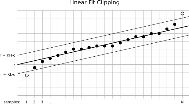
In this figure we have the same set of pixels as before. However, the linear fit clipping algorithm is being used instead of sigma clipping. The new algorithm fits a straight line to the set of pixels. It tries to find the best possible fit in the sense of minimizing average deviation. Average deviation is computed as the mean of the distances of all pixel values to the line. When we find a line that minimizes average deviation, what we have found is the actual tendency in the set of pixel values. Note that a linear fit is more robust than a sigma clipping scheme, in the sense that the fitted line does not depend, to a larger extent, on all the images having flat illumination profiles. If all the images are flat (and have been normalized, as part of the rejection procedure), then the fitted line will tend to be horizontal. If there are illumination variations, then the line's slope will tend to grow. In practice, a linear fit is more tolerant to slight additive gradients than sigma clipping.
The neat result is that less false outliers are being rejected, and hence more pixels will enter the final integrated image, improving the SNR. In the figure, r is the fitted line and d represents average absolute deviation. KH and KL, as before, are two multipliers for high and low pixels, but this time they are expressed in average absolute deviation units. Instead of classifying pixels with respect to a fixed value (the median in the case of sigma clipping), in the linear fit algorithm low and high pixels are those that lie below and above the fitted line, respectively. Note that in the linear fit case only two pixels have been rejected as outliers, while the set of inlier pixels fit to a straight line really well. In addition, the employed tolerance is more restrictive in the linear fit case ?compare d with sigma on the two preceding figures.
The remaining question is: is linear fit clipping the best rejection algorithm? I wouldn't say that as a general statement. Linear fit rejection requires a relatively large set of images to work optimally. With less than 15 images or so its performance may be worse or similar to Winsorized sigma clipping. To reject pixels around a fitted line with low uncertainty, many points are required in order to optimize it in the least average absolute deviation sense. The more images, the better linear fit is possible, and hence the new algorithm will also perform better. It's a matter of testing it and see if it can yield better results than the other rejection algorithms available, for each particular case.
Rejection Maps and the Slope Map
The linear fit clipping rejection algorithm generates, when the Generate rejection maps option is enabled, a slope map image along with the standard low and high rejection maps.
Pixels in a rejection map have values proportional to the number of rejected pixels in each stack of pixels. For example, if a rejection map pixel is white (with a value of 1.0), that means that all pixels have been rejected at its image coordinates in the set of integrated images. A black rejection map pixel (= 0.0) means that no pixel has been rejected, and intermediate values 0 < x < 1 represent the amount of rejected pixels. Rejection maps have many interesting applications. The most obvious is evaluating the quality and suitability of a pixel rejection process. For example, it is easy to know if some plane trails or cosmic rays have been properly rejected by just inspecting the high rejection map at the appropriate locations.
A slope map represents the variations in each pixel stack, as evaluated by the linear fit clipping algorithm. A pixel in a slope map has a value proportional to the slope of the fitted line for the corresponding pixel stack. Recall that the slope of a line that passes through two points {x1,y1} and {x2,y2} on the plane is the quotient between the vertical and horizontal increments, that is: slope = (y2-y1)/(x2-x1).
Thus a slope map value of 0 means that all the pixels in the corresponding stack have the same value (on average), since the fitted line is horizontal (slope = 0) in this case. A slope value of 0.5 corresponds to a slope angle of 45 degrees, which is very high (you rarely will see it). A slope value of 1.0 would correspond, in theory, to infinite slope, or a fitted line that would form an angle of 90 degrees with respect to the X axis ?which is impossible, for obvious reasons.
In the screenshot at the beginning of this post, which I'll repeat below for your convenience, you can see a slope map generated after integration of 19 images with the new linear fit clipping rejection algorithm. It is the image with the 'slope' identifier.
Along with the slope map, you can see also the standard 'rejection_low' and 'rejection_high' maps. Note that the three map images have active screen transfer functions (STF) applied, so their actual values are being largely exaggerated on the screenshot.
In the set of 19 integrated images, approximately one half of them have additive sky gradients that are brighter toward the top of the frame, and the other half has the opposite gradients: brighter toward the bottom of the frame. Note how the slope map has represented these variations, as both the top and bottom parts of the map image are brighter on the sky background. Note also that the main objects M81 and M82, as well as most bright stars, are being represented as having relatively strong variations on the slope map. This is normal and happens quite frequently. It means that in the set of integrated images, there are significant variations due to varying atmospheric conditions, different exposure times, and other factors.
Slope maps represent a new tool available in PixInsight for controlling the properties of the image integration process. We haven't designed any specific application for these maps yet, but following the design principles and philosophy that govern PixInsight, we provide you with new tools and resources that maximize your control over everything that happens with your data. This is the PixInsight way that you love")
Persistent File Cache
Another important new feature of ImageIntegration is a persistent file cache. ImageIntegration has already had an efficient file cache since its first version. The cache stores a set of statistical data for each integrated image, which are necessary to perform the integration task, such as the extreme pixel values, the average value, the median, some deviations, noise estimates, etc. Calculation of all of these data is quite expensive computationally. By storing these data in a cache, ImageIntegration can run much faster because if you repeat the integration procedure with the same images, for example to try out new pixel rejection parameters, ImageIntegration can retireve the necessary data from the cache, avoiding a new calculation.
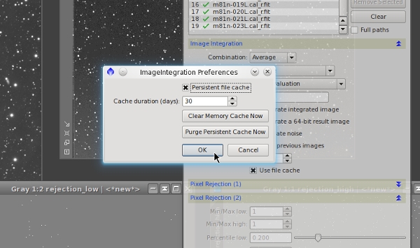
In previous versions of the ImageIntegration tool, the cache was volatile, that is, it was lost when you terminated the current PixInsight session. The new cache is persistent, which means that it is remembered across PixInsight sessions. In the screenshot below you can see the new dialog box that allows you to control the persistent cache with several options.
A similar cache will also be available for StarAlignment in one of the next 1.6.x versions. In this case, the persistent cache will store all stars detected in each image, which will speed up the image registration process very significantly.
The latest version 1.6.1 of PixInsight comes with a couple new features implemented in the ImageIntegration tool. This is a brief description of both, where I'll borrow some figures and text from other posts to make up a sort of official description.
Linear Fit Clipping Pixel Rejection Algorithm
The new Linear Fit Clipping rejection method fits the best possible straight line, in the twofold sense of minimizing average deviation and maximizing inliers, to the set of pixel values in each pixel stack. At the same time, all pixels that don't agree with the fitted line (to within user-defined tolerances) are considered as outliers and thus rejected to enter the final integrated image.
The new pixel rejection algorithm is controlled, as usual, with two dedicated threshold parameters in sigma units: Linear fit low and Linear fit high, respectively for low and high pixels. The screenshot below shows the new version of ImageIntegration and some results of the new rejection method.
The difference between linear fit clipping and sigma clipping is best explained with a graphical example. Consider the following figure.
Suppose we are integrating N images. In the figure, we have represented a stack of N pixels at the same coordinates, whose values have been sorted in ascending order and plotted as circles on the graphic. The horizontal axis is the ordered sample number, and the vertical axis represents the available range of pixel values.
What we pursue with pixel rejection is to exclude those pixels that have spurious values, such as pixels pertaining to cosmic rays, plane and satellite trails, and other too high or too low pixels that are not valid data for some reason. We want to reject those pixels to make sure that they won't enter the integrated image.
The symbol m represents the median of the distribution. The median is the value of the central element in the ordered sequence, which in statistical terms corresponds to the most probable value in the distribution. Here, the median is being used as a robust estimate of the true value of the pixel, or more realistically, the most representative value of the pixel that we have available. Robustness here means unaffected by outliers. An outlier is a value abnormally low or high, as are both extreme values in the graphic, for example. Outliers are precisely those values that we want to exclude, or reject. By contrast, valid pixel values or inliers are those that we want to keep and integrate as a single image to achieve a better signal-to-noise ratio. Our goal is to reject only really spurious pixels. We need a very accurate method able to distinguish between valid and not valid data in a smart way, adapted to the variety of problems that we have in our images. Ideally no valid data should be rejected at all.
With two horizontal lines we have represented the clipping points for high and low pixels, which are the pixels above and below the median of the stack, respectively. Pixels that fall outside the range defined by both clipping points are considered as outliers, and hence rejected. In the sigma clipping algorithm, as well as in its Winsorized variant, clipping points are defined by two multipliers in sigma units, namely KH and KL in the figure. Sigma is an estimate of the dispersion in the distribution of pixel values. In the standard sigma clipping algorithms, sigma is taken as the standard deviation of the pixel stack. These algorithms are iterative: the clipping process is repeated until no more pixels can be rejected.
In the figure, rejected pixels have been represented as void circles. Six pixels have been rejected, three at each end of the distribution. The question is, are these pixels really outliers? The answer is most likely yes, under normal conditions. Normal conditions include that the N images have flat illumination profiles. Suppose that some of the images have slight additive sky gradients of different intensities and orientations ?for example, one of the images is slightly more illuminated toward its upper half, while another image is somewhat more illuminated on its lower half. Or, for example, that some of the images have been acquired under worse transparency conditions. Due to varying gradients and illumination levels, the sorted distribution of pixels can show tails of apparent outliers at both ends. This may lead to the incorrect rejection of valid pixels with a sigma clipping algorithm.
Enter linear fit clipping:
In this figure we have the same set of pixels as before. However, the linear fit clipping algorithm is being used instead of sigma clipping. The new algorithm fits a straight line to the set of pixels. It tries to find the best possible fit in the sense of minimizing average deviation. Average deviation is computed as the mean of the distances of all pixel values to the line. When we find a line that minimizes average deviation, what we have found is the actual tendency in the set of pixel values. Note that a linear fit is more robust than a sigma clipping scheme, in the sense that the fitted line does not depend, to a larger extent, on all the images having flat illumination profiles. If all the images are flat (and have been normalized, as part of the rejection procedure), then the fitted line will tend to be horizontal. If there are illumination variations, then the line's slope will tend to grow. In practice, a linear fit is more tolerant to slight additive gradients than sigma clipping.
The neat result is that less false outliers are being rejected, and hence more pixels will enter the final integrated image, improving the SNR. In the figure, r is the fitted line and d represents average absolute deviation. KH and KL, as before, are two multipliers for high and low pixels, but this time they are expressed in average absolute deviation units. Instead of classifying pixels with respect to a fixed value (the median in the case of sigma clipping), in the linear fit algorithm low and high pixels are those that lie below and above the fitted line, respectively. Note that in the linear fit case only two pixels have been rejected as outliers, while the set of inlier pixels fit to a straight line really well. In addition, the employed tolerance is more restrictive in the linear fit case ?compare d with sigma on the two preceding figures.
The remaining question is: is linear fit clipping the best rejection algorithm? I wouldn't say that as a general statement. Linear fit rejection requires a relatively large set of images to work optimally. With less than 15 images or so its performance may be worse or similar to Winsorized sigma clipping. To reject pixels around a fitted line with low uncertainty, many points are required in order to optimize it in the least average absolute deviation sense. The more images, the better linear fit is possible, and hence the new algorithm will also perform better. It's a matter of testing it and see if it can yield better results than the other rejection algorithms available, for each particular case.
Rejection Maps and the Slope Map
The linear fit clipping rejection algorithm generates, when the Generate rejection maps option is enabled, a slope map image along with the standard low and high rejection maps.
Pixels in a rejection map have values proportional to the number of rejected pixels in each stack of pixels. For example, if a rejection map pixel is white (with a value of 1.0), that means that all pixels have been rejected at its image coordinates in the set of integrated images. A black rejection map pixel (= 0.0) means that no pixel has been rejected, and intermediate values 0 < x < 1 represent the amount of rejected pixels. Rejection maps have many interesting applications. The most obvious is evaluating the quality and suitability of a pixel rejection process. For example, it is easy to know if some plane trails or cosmic rays have been properly rejected by just inspecting the high rejection map at the appropriate locations.
A slope map represents the variations in each pixel stack, as evaluated by the linear fit clipping algorithm. A pixel in a slope map has a value proportional to the slope of the fitted line for the corresponding pixel stack. Recall that the slope of a line that passes through two points {x1,y1} and {x2,y2} on the plane is the quotient between the vertical and horizontal increments, that is: slope = (y2-y1)/(x2-x1).
Thus a slope map value of 0 means that all the pixels in the corresponding stack have the same value (on average), since the fitted line is horizontal (slope = 0) in this case. A slope value of 0.5 corresponds to a slope angle of 45 degrees, which is very high (you rarely will see it). A slope value of 1.0 would correspond, in theory, to infinite slope, or a fitted line that would form an angle of 90 degrees with respect to the X axis ?which is impossible, for obvious reasons.
In the screenshot at the beginning of this post, which I'll repeat below for your convenience, you can see a slope map generated after integration of 19 images with the new linear fit clipping rejection algorithm. It is the image with the 'slope' identifier.
Along with the slope map, you can see also the standard 'rejection_low' and 'rejection_high' maps. Note that the three map images have active screen transfer functions (STF) applied, so their actual values are being largely exaggerated on the screenshot.
In the set of 19 integrated images, approximately one half of them have additive sky gradients that are brighter toward the top of the frame, and the other half has the opposite gradients: brighter toward the bottom of the frame. Note how the slope map has represented these variations, as both the top and bottom parts of the map image are brighter on the sky background. Note also that the main objects M81 and M82, as well as most bright stars, are being represented as having relatively strong variations on the slope map. This is normal and happens quite frequently. It means that in the set of integrated images, there are significant variations due to varying atmospheric conditions, different exposure times, and other factors.
Slope maps represent a new tool available in PixInsight for controlling the properties of the image integration process. We haven't designed any specific application for these maps yet, but following the design principles and philosophy that govern PixInsight, we provide you with new tools and resources that maximize your control over everything that happens with your data. This is the PixInsight way that you love
Persistent File Cache
Another important new feature of ImageIntegration is a persistent file cache. ImageIntegration has already had an efficient file cache since its first version. The cache stores a set of statistical data for each integrated image, which are necessary to perform the integration task, such as the extreme pixel values, the average value, the median, some deviations, noise estimates, etc. Calculation of all of these data is quite expensive computationally. By storing these data in a cache, ImageIntegration can run much faster because if you repeat the integration procedure with the same images, for example to try out new pixel rejection parameters, ImageIntegration can retireve the necessary data from the cache, avoiding a new calculation.
In previous versions of the ImageIntegration tool, the cache was volatile, that is, it was lost when you terminated the current PixInsight session. The new cache is persistent, which means that it is remembered across PixInsight sessions. In the screenshot below you can see the new dialog box that allows you to control the persistent cache with several options.
A similar cache will also be available for StarAlignment in one of the next 1.6.x versions. In this case, the persistent cache will store all stars detected in each image, which will speed up the image registration process very significantly.