1 Introduction
[hide]
Image acquisition with an electronic sensor, whether a CCD or a CMOS, is based on the absorption of light by the sensor's surface and the consequent generation of an electrical signal, in the form of electrons, thanks to the photoelectric effect [1]. The photoelectric effect tells us that light is composed of particles, called photons, capable of interacting with matter: if the photon has enough energy, it will kick off the electron out of its original position giving it the ability to move away.
A digital image sensor is a bi-dimensional array of photosites. Photosites are like buckets that convert incident light into electrons and trap them in place: the produced photocurrent is therefore integrated into electrical charge. After exposure, the generated electrical charge of each photosite converts to voltage in the readout process. Each voltage is amplified and then converted to a number by a device known as analog–to–digital converter (A/D converter, or ADC). Therefore each photosite is represented as a single picture element, or pixel, in the final 2D array of values that makes the image: the intensity unit is called Analog to Digit Unit or ADU. The conversion constant between electrons and ADU is called gain, so there is only a multiplicative factor between the two values.
An essential feature of a good digital image sensor is that the amount of charge collected by each photosite is directly proportional, through a linear relationship, to the amount of light that hit it: in other words, if the intensity of the light doubles then the final charge will double, or if the exposure time doubles, keeping the same light flux, again, the final charge will double. This feature is called sensor linearity and is a fundamental property underlying the theory of image calibration.
1.1 Calibration basics
The output charge depends only on the light intensity (photon flux) and exposure time in an ideal image sensor attached to an ideal optical train. As explained before, this charge distribution is transformed into an image thanks to the ADC.
Below we'll refer to this ideal image as  .
.
In the actual case, the situation is more complicated: other phenomena contribute to the amount of final charge of a photosite.
- The optical train may change the photons flux due to geometrical and optical effects that produce uneven sensor illumination. The effect is different in different places on the sensor surface, creating the well-known effect called vignetting.
- Dust particles may settle on the sensor window or the filter's surface, casting shadows on the underlying photosites. An off-axis guider mirror may also cast shadows. All these effects reduce the number of photons hitting the sensor.
- Not all the photons that reach a photosite produce a photoelectron: the probability that a photon can produce an electron is called quantum efficiency (QE): A QE of 75% means that, on average, out of 100 photons incident on a photosite, only 75 will produce a photoelectron. The average value of QE of an image sensor depends mainly on the wavelength of the light, but slight differences in QE may be possible in nearby photosites; this means that, even with uniform illumination, nearby pixels may show different average ADU values.
- Thermal energy can kick off electrons from their position, just like photons. These thermal electrons are trapped in photosites even when the sensor is not illuminated; this is why we refer to this additional signal as dark current. Thermal electrons add up to the photo-electrons in the photosite: since electrons are identical particles, photo-electrons are indistinguishable from thermal ones and produce together the overall charge trapped in the photosite. The dark current amount depends mainly on sensor temperature and exposure time.
- For technical reasons beyond this documentation's scope, an artificially induced electronic offset is introduced in the photosites; this ensures that the Analog-to-Digital Converter (ADC) always receives a positive signal. Moreover, further charges can be generated during the photosite reading phase, adding to the standard offset. This zero signal charge is usually called bias.
Points 1, 2 and 3 cause the loss of a certain percentage of photons with respect to the hypothetical value; hence they can be accounted with a single multiplicative factor that depends on the position on the sensor surface:  , where
 and
and  stand for quantum efficiency, vignetting and shadowing, respectively.
Points 3 and 4 produce an additive signal added as a variable offset to the genuine photon-related signal.
Now the interesting linearity property of the sensor comes into play: remembering that the number of photo-electrons is directly proportional to photon flux and that it can be easily converted to intensity through the gain value, we can write
 [1]
[1]where
 is, as explained before, the intensity expected just before entering inside the telescope: this would be the image we would get if the shooting system (telescope plus camera) were perfect. It depends on the given position
  on the sensor' surface and on the gain
 is the intensity measured in a given position on the sensor' surface for a given gain
  Is the multiplicative factor in a given position that accounts for QE variations, vignetting and shadowing: it is normalized between 0 and 1 where 0 means that no photons are detected in a certain pixel.
 Is the dark current in a given position on the sensor' surface, for an exposure time
  and a temperature
 Is the bias in a given position on the sensor' surface, with a given temperature
  and given Offset and gain
  and
and
For the sake of readability, in equation [1] we can imply dependencies on position, exposure time, temperature, and gain, writing a simplified version:
 [2]
[2]1.2 Artifacts
Besides the phenomena already analyzed, other factors contribute to the appearance of the output frame, all additive in nature:
- Hot pixel
- Cold pixel
- Defective rows/columns
- Amp-glow
Hot pixels are produced by individual photosites with higher-than-normal dark current rates. They appear as abnormally bright pixels on long-exposure images.
Cold pixels are produced by individual photosites with lower-than-normal sensitivity (even as low as zero, known as a dead pixel). They appear as abnormally dark pixels in otherwise bright areas of an image.
Defective rows/columns are just rows/columns of pixels that do not work properly; some columns are entirely "dead" (dark), some are "hot" (bright), some have just a constant added to what they should normally show.
Traps. Some pixels are defective and cannot transfer electrons when the image is read out. All the pixels below such a bad pixel will be normal, but all those above it are lost because their electrons are trapped in the bad pixel; this forms a partially bad column.
All the above artifacts are generally called cosmetic defects (See also the CosmeticCorrection process).
Amp-glow is an artifact appearing as bright spots on the image, usually in the corners or along the borders. In CCD cameras, amp-glow is caused by an infrared glow coming from the amplifier that converts electrons into voltage. CMOS sensors don't have a single amplifier like CCDs, but various circuits can produce such a glow, caused both by a thermal phenomenon or by infrared light production.
As mentioned above all these artifacts are additive and are present in the dark frame. They can be considered included in the  component in equation [2].
1.3 Noise
Noise is a crucial topic in digital photography in general and in astrophotography in particular, where weak signals are particularly affected by this phenomenon. Image noise is a variation in pixel brightness not correlated with the input signal. Image noise is an undesirable by-product of image acquisition that may hide the desired information.
There are common misunderstandings about the role of calibration in noise handling; therefore, some fundamental concepts need to be pointed out.
We can divide noise sources into two main types: [5] temporal noise and fixed-pattern noise.
1.3.1 Temporal noise
Temporal noise is the temporal variation in pixel output values under constant illumination due to device noise, supply and substrate noise, and quantization effects.[5] (lecture 6)
In this sentence the word temporal means "while time goes by": repeated readings of a single pixel give different values varying around an average level. This random variation from frame to frame is called temporal noise.
Temporal noise, therefore, appears as a random grainy effect on the image, mainly in the darker areas, whose spatial structure changes from frame to frame.
The main sources of temporal noise are:
- Thermal noise, or dark noise.
- Readout noise.
- Shot noise.
An essential property of temporal noise is that it cannot be removed through calibration. On the contrary, the calibration process adds the noise of the calibration frames to the noise in the images being calibrated. This is why master calibration frames composed of many subframes are needed: the only way to reduce temporal noise is by integrating many images.
1.3.2 Fixed pattern noise
Fixed-pattern noise (FPN), also called nonuniformity, is the spatial variation in pixel average output values under uniform illumination due to device and interconnect parameter variations (mismatches) across the sensor.[5] (lecture 7)
FPN is generated by imperfections of the sensor: the individual photosites in a sensor do not behave ideally. There are pixel-to-pixel variations in bias offset, dark current and light sensitivity.
The effect of FPN may be negligible in daylight photography, but it is crucial in low-light photography, particularly in astrophotography. Whereas temporal noise can be reduced by capturing and integrating more frames, FPN cannot be reduced this way. On the contrary, FPN has to be removed as far as possible from individual frames, or it will become visible once the image is stretched nonlinearly to make it visible. FPN will emerge even more clearly in deeper exposed images.
Luckily, even if the FPN has a random pattern on the image sensor, its structure is stable in time; it is, therefore, present in calibration frames and can be removed easily.
1.4 Types of calibration frames
1.4.1 Bias frame
Bias frames are captured with the sensor in complete darkness at the shortest exposure time that the camera can provide, which is achieved by setting an exposure time of zero seconds. The bias signal contains only the constant bias offset and the additive fixed pattern noise generated in the readout process.
Bias frames are needed when dark frame optimization shall be applied. Bias frames are also needed for the calibration of shortly exposed flat frames which, usually, do not contain a significant amount of dark signal.
Please note: The bias frames of cameras with a Panasonic MN 34230 sensor show a varying gradient across the frame and an inconsistent bias level when exposure times < 0.2 s are used[4]. With such a camera, it is not advisable to use bias frames at all. Another sensor that seems to show a similar behavior is the Sony IMX294. However, it is not valid to generalize this recommendation for all CMOS sensors: other CMOS sensors may not show this anomaly of an inconsistent bias level.
Since both the light component and the dark current are zero (no light and zero exposure time), equation [2] takes the very simple form
 [3]
[3]where  is the bias frame.
1.4.2 Dark frame
Dark frames are captured with the sensor in complete darkness at an exposure time that matches the frames they are intended to calibrate (the target frames). In the special case when dark frame optimization shall be applied for calibration of the target frames, the exposure time of the dark frames should be greater than or equal to the exposure time of the target frames.
Since the light component is zero (no light), and considering equation [3], equation [2] takes the form
 [4]
[4]where  is the dark frame.
A dark frame, therefore, contains both the bias and dark signals. The dark signal consists of the term dark current × exposure time and the fixed defects described in the artifacts paragraph.
A special kind of dark frame is the flat-dark. Flat-darks are captured with the sensor in complete darkness at the same exposure time as the flat frames.
For a rigorous calibration practice (i.e., scientific-grade calibration), flat-darks shall always be used to calibrate flat frames. From a practical point of view, however, the dark signal in a flat frame is usually negligible because exposure times are short. In these cases, if the camera does not suffer from bias level instability,[4] the bias frame can be used instead of a flat-dark frame.
A second valid technique is using a dark frame with a longer exposure time, using the dark frame optimization feature.
It is essential to point out that these flat-dark surrogates should be used only after a direct comparison with a real flat-dark to assess that the differences are negligible.
1.4.3 Flat frame
Flat frames are captured through the telescope or lens, and it is essential that the field be as evenly illuminated as possible. In this case, equation [2] takes the form
 [5]
[5]where  is the flat-dark frame that usually can be replaced with the bias frame, or an optimized dark frame, as explained before, and
  is a constant value on the whole sensor surface.
As we'll explain below, flat frames must be calibrated before integrating them into the master flat frame, which will be applied later to the dark-calibrated light frames during image calibration.
Thus, flat frames are necessary for the correction of vignetting, shadowing effects caused by dust particles, and the fixed pattern generated by differences in light sensitivity of individual photosites in a sensor. It also corrects for the multiplicative component of fixed pattern noise. This step of the calibration process is called flat field correction.
1.4.4 The master calibration frames
As explained in the noise paragraph, temporal noise cannot be removed from frames: during the calibration phase, the temporal noise in the calibration frames adds up to the noise already present in the images. The only way to reduce this calibration drawback is to reduce the temporal noise by averaging many single calibration frames. this integration has two effects:
- It reduces the temporal noise component approximately by
 , where
  is the number of single frames averaged.
 - It gives a better estimate on the fixed pattern noise component.
These images are the master calibration frames.
-
Uncalibrated master bias
-
Obtained by averaging the bias frames.
-
Uncalibrated master dark/flat-dark
-
Obtained by averaging the dark frames. It is uncalibrated because it contains the bias signal.
-
Master Flat
-
Obtained by averaging the flat frames after calibration with an uncalibrated master flat-dark.
Important note— A few tutorials recommend using calibrated versions of the master bias and master dark frames.
The bias frame can be calibrated via the overscan area if present, the calibrated master dark is then obtained averaging the dark frames after calibration with a master bias or via the overscan area: it contains only the dark current information and some additive artifacts.
Anyway, if the dark current is very low, calibrating the dark frames without a proper additive pedestal could lead to data clipping at zero and cause an incorrect noise evaluation; therefore, calibrating the bias and the dark frames is not a recommended calibration practice.
1.5 The calibration equation
The purpose of the calibration procedure is to reverse the effects of the image acquisition system, removing both additive and multiplicative effects thanks to appropriate calibration frames.
Equation [2] can be simply inverted to obtain  :
:
 [6]
[6]The multiplicative factor can be derived from equation [5]:
 [7]
[7]In the above equations an uncalibrated master dark  may be used for the
  component, and a calibrated master flat
  may be used for the
  component. Merging equations [6] and [7], the main calibration equation can be written as
 [8]
[8]where is the flat scaling factor. In PixInsight,  , so the mean value of the calibrated light frame doesn't change after flat field correction.
1.6 The dark frame optimization
Equation [8] assumes that the master dark has been acquired with the sensor at the same temperature and with the same exposure time as the light frame to be calibrated. In other words, that the dark current signal in the dark frame perfectly matches the dark current signal in the light frame. This is not always true: sometimes temperature control is missing or subject to fluctuations, and sometimes a dark frame with the exactly matching time is missing. In general, the actual problem is more complex because the dark current is highly time- and temperature-dependent, so a perfect match between the dark current signals in  and is only a theoretical goal.
A better, even if not perfect, approach is to split the dark frame contribution into dark current and bias, applying a scaling factor  that attempts to account for effective exposure time and temperature differences between the light frame and the master dark frame.
Using an uncalibrated master dark and a master bias  , equation [8] becomes:[7]
 [9]
[9]where is the dark frame optimization factor. If the master dark perfectly matches the light frame, we have  and equation [9] reduces to equation [8].
The dark frame optimization problem is a relatively simple case of function optimization with a single parameter. The first step is therefore to define the cost function that we want to minimize. To explain why and how we have selected a particular function we need some visual analysis. Take a look at the following two images:
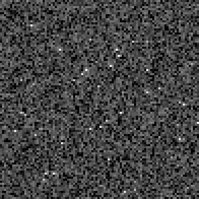
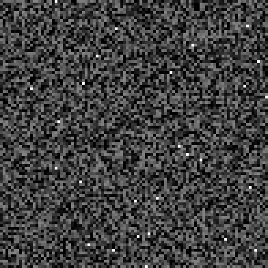
The image on the left is a bias-subtracted master dark frame, while the image to the right is a mix of synthetically generated uniform noise and impulsional noise (salt-and-pepper noise)[2] with 0.5% probability. This comparison shows that a master dark frame looks very similar to random noise. Essentially, a master dark frame is composed of pixel-to-pixel intensity variations whose spatial distribution is rather uniform, plus a relatively small amount of hot pixels whose distribution and typical values are similar to impulsional noise. Of course, we know that the thermal noise is a fixed pattern characteristic of a given sensor, so it is not random, being predictable. However, morphologically a master dark frame is virtually indistinguishable from random noise.
The cost function to be minimized is, essentially, a noise evaluation function. This can be implemented applying an iterative k-sigma noise estimation algorithm[8] on the calibrated image, or simply by estimating a robust variance. As explained before, in fact, the master dark contains mainly fixed pattern noise (FPN); when the optimized master dark matches the light frame the optimized FPN elides the FPN in the light frame and the noise evaluation function reaches a minimum.
The rest of the algorithm, therefore, is a routine to find the minimum of a unimodal function, using an adaptation of the classical golden section search algorithm.[3]
Summarizing, the algorithm can be described at the high level as follows:
- Find a range
 of dark scaling factors that brackets the minimum of the noise evaluation function. This is the initial bracketing phase.
 - Iterate the golden section search algorithm to find the minimum of the noise evaluation function
 . At each iteration, compute the calibrated raw frame as:
  and evaluate the noise in
  .
. - Iterate until the minimum of the noise evaluation function is determined up to a prescribed accuracy (1/1000 fractional accuracy in our implementation).
- The final value of the dark scaling factor is the value of from the last iteration.
This algorithm has proven extremely robust and accurate. However it has two known problems:
- It is very sensitive to bad-quality calibration frames. In particular, if the master bias and/or the master dark frames include significant amounts of temporal noise, the optimization algorithm will find a value of that overcorrects thermal noise to compensate for the additive random noise component. In extreme cases, this may lead to dark holes as a result of overcorrected hot pixels.
- It implicitly assumes that the dark optimization function is constant for the whole range of numerical data values, since it consists of a simple multiplicative factor. This is not the case in practice, especially for high-intensity values. As a result of this simplistic optimization model, the algorithm tends to undercorrect hot pixels. This is a very minor issue, however, since hot pixels are easily rejected during integration (assuming that all frames have been correctly dithered) and can be removed also with cosmetic correction techniques, if necessary.
Whether it is favourable to use dark frame optimization or not depends essentially on camera characteristics. Using dark frame optimization for a camera without temperature control may significantly improve the calibration result; this is because temperature deviations between dark and light frame acquisition are unavoidable in this case. For a camera with temperature control the benefit of dark frame optimization will be much smaller, possibly even not detectable.
However, if the sensor shows "amplifier glow", this might not be calibrated out completely with dark frame optimization enabled. In the case of a camera without temperature control and with "amplifier glow" it's worthwhile to accurately compare the results of both settings (compare the final integration results after image calibration, demosaicing if applicable, and registration of the light frames).
Read the section How to verify the optimization performance for further information on how to verify if a camera is suitable for dark frame optimization.
Even if, in general, the optimization algorithm can work with any combination of dark and light frames, it is a better calibration practice using a master dark with a longer exposure time or a higher temperature compared to the light frame. The scaling factor , in fact, multiplies both the dark current and the temporal noise in the master dark. Using a master dark with a shorter exposure time leads to  , which increases the temporal noise in the final calibrated image.
2 Parameters
[hide]
2.1 Target frames
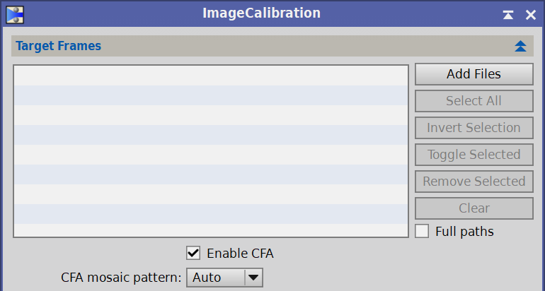
Use these controls to define and manage a list of image files to be calibrated.
-
The largest control in this section is a list box with all the images currently selected for calibration. The list will show full file paths or just file names, depending on the state of the Full Paths checkbox. You must select at least one file. On this list you can:
- Double-click an item's file name or path to open it in PixInsight as a new image window.
- Double-click a green checkmark icon to disable an item (double-click the red crossmark icon to enable it). Disabled files will not be calibrated.
-
Add Files
-
Click this button to open a file dialog where you can select new image files that will be appended to the current list of target images to be integrated. Only files located in the local filesystem can be selected; the tool does not currently support remote files located on network devices.
-
Select All
-
Click this button to select all the files in the current list of input images.
-
Invert Selection
-
Click this button to invert the current selection in the list of input images.
-
Toggle Selected
-
Click this button to enable/disable the files currently selected in the list of input images.
-
Remove Selected
-
This button removes the selected files from the list of input images. This action cannot be undone.
-
Clear
-
Click to empty the list of input images. This action cannot be undone.
-
When this option is selected, the list of input files will show each selected image's full absolute file paths. When this option is disabled (default state), only file names will be shown, which simplifies visual inspection, and full file paths are shown as tooltip messages.
-
Enable CFA
-
Activate the Color Filter Array (CFA) mode.
Dark frame optimization of CFA images, such as Bayerized DSLR or OSC raw images, requires a previous demosaicing step in order to compute valid noise estimates. The resulting CFA mode is also used to calculate the noise if Noise evalutation was selected. It is recommended to use Force CFA or the cfa input hint if you haveCFA files to avoid any error in noise evaluation.
CFA mode it is also used to calculate Separate CFA scaling factors for the flat field calibration.
-
CFA mosaic pattern
-
This parameter defines how CFA patters are handled for computation of master dark and master flat scaling factors.
The Auto option uses view properties that can be available in the master and target frame files. Under normal condition s, these properties are either generated automatically by the RAW format support module and stored in XISF files, or available as FITS header keywords in the case of RAW OSC frames.
For non-CFA data acquired with monochrome cameras, the Auto option is the correct selection because in these cases the process will detecto no CFA pattern.
For images acquired with X-Trans sensors this parameter is ignored and CFA patterns are always extracted from existing image properties.
2.2 Format Hints
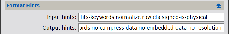
Format hints are small text strings that allow you to override global file format settings for image files used by specific processes. In the ImageCalibration tool, input hints change the way input images of some particular file formats are loaded during the calibration process, while output hints modify how output calibrated frames are written.
The default input hints are:
- fits-keywords
-
Read/write FITS header keywords in XISF format, for legacy format compatibility.
- normalize
-
Normalize floating point real pixel data to the [0,1] range. Normalize integer data to [0,2 n–1].
- raw
-
Load a raw Bayer RGB image without interpolation, no white balancing, no black point correction, with unused frame areas cropped, no frame rotation, no highlights clipping, and no noise reduction.
- cfa
-
Load a monochrome raw CFA frame.
- signed-is-physical
-
Signed integer images store physical pixel data in the range [0,+2n–1–1], where n is bit depth.
The default output hints are:
- properties
-
Read/write image and unit properties.
- fits-keywords
-
Read/write FITS header keywords in XISF format, for legacy format compatibility.
- no-compress-data
-
Do not generate compressed data blocks.
- no-embedded-data
-
Do not read/write embedded image data.
- no-resolution
-
Do not generate image resolution metadata.
Most standard file format modules support hints; each format supports a number of input and/or output hints that you can use for different purposes with tools that give you access to format hints. A full list of format hints for each file format are available in the Format Explorer, selecting the desired format and double clicking the Implementation row.
In the format hints list, after the hint name, an (r ) means that it is an input hint, a ( w) means that it is an output hint, a (rw) means that it can be both input ands output.
2.3 Output Files
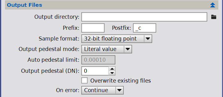
This section allows to define important parameters to control generation of calibrated image.
-
Output directory
-
This is the directory (or folder) where all output files will be written. If this field is left blank (the default value), each output file will be written to the same directory of its corresponding target frame file. In such case, make sure that source directories are writable, or the calibration process will fail upon trying to create the first output file.
-
Output prefix
-
This is a short piece of text that will be prepended to the file names of all output calibrated images. For example, if a target image is "myBestImage.xisf" and you specify "cal_" as a prefix, the corresponding output file will be "cal_myBestImage.xisf". Specifying file prefixes and/or postfixes, along with the use of a specific directory for each task, are good practices to keep your working data well organized. With large data sets these practices can become extremely important.
The default value of this parameter is an empty string, so no output prefix is used by default.
-
Output postfix
-
This is a short piece of text that will be appended to the file names of all output calibration images. For example, if a target image is "myBestImage.xisf" and you specify "_cal" as a postfix, the corresponding output file will be "myBestImage_cal.xisf". Specifying file prefixes and/or postfixes, along with the use of a specific directory for each task, are good practices to keep your working data well organized. With large data sets these practices can become extremely important.
The default value of this parameter is "_c", so this is the postfix added to all output files by default. Other tools use different file postfixes; for example, the standard StarAlignment tool uses the "_r" postfix. This helps you identify the working data being generated at each stage of your preprocessing procedures.
-
Sample format
-
This is the pixel sample format used to generate all output calibrated images. :
-
16-bit integer
-
Writes all output calibrated images in 16-bit unsigned integer format (0 to 65535 range). Warning: With the exception of some special control and diagnostics tasks, this option should never be used for production work.
-
32-bit integer
-
Writes all output calibrated images in 32-bit unsigned integer format (0 to 232–1 range).
-
32-bit floating point
-
Writes all output calibrated images in 32-bit IEEE 754 floating point format.
-
64-bit floating point
-
Writes all output calibrated images in 64-bit IEEE 754 floating point format.
The default value of this paramter is 32-bit floating point.
-
-
The output pedestal is a small quantity expressed in the 16-bit unsigned integer range (from 0 to 65535). It is added at the end of the calibration process, and its purpose is to prevent negative values that can sometimes occur due to overscan and bias subtraction. Under normal conditions, you should need no pedestal to calibrate science frames because mean sky background levels should be sufficiently high to avoid negative values. Sometimes, a small pedestal can be necessary to calibrate individual bias and dark frames.
Another case where a small output pedestal could be helpful is when imaging with narrowband filters under very dark skies; in these situations, the mean level of the sky background could be near to the dark frame level and, without a small pedestal, negative values, clipped to zero, may arise.
The pedestal value must be high enough to prevent data clipping but not too high because it might reduce the image dynamic range; its value must be chosen carefully.
This parameter defines how ImageCalibration handles the pedestal.
-
Literal value
-
It allows to manually define a pedestal value in 16-bit data number units (DN) using the output pedestal parameter.
-
Automatic
-
It automatically defines the pedestal value based on a statistical analysis of the image. ImageCalibration calculates the pedestal value only for frames that, after all the calibration steps, have negative or insignificant (to machine epsilon) minimum pixel values. The automatic pedestal is computed individually for each frame as a statistically significant, robust mean value to ensure the positivity of the calibrated image with minimal truncation.
If the pedestal, automatic or literal is different than zero, than a keyword PEDESTAL is added to the calibrated file header.
-
-
This parameter defines the the maximum allowed fraction of negative or insignificant pixels allowed in automatic pedestal mode; when, after calibration, the image has more than this fraction of negative or insignificant pixel and the Output pedestal mode is set to Automatic, the process will compute the automatic pedestal as a robust, statistically significant additive value to ensure positivity of the calibrated image with minimal truncation (the expected tuncation is the Limit value in the [0,1] range).
The default limit value is 0.0001 which represents 0.1% of the whole image pixels.
-
If the Output pedestal mode is set to Literal value this is the value of the pedestal added to every frame processed by ImageCalibration.
The pedestal is expessed in 16-bit data number units (DN).
The default value is zero, if a different value is specified the kewyword PEDESTAL is added to the calibrated file HEADER.
-
Overwrite existing files
-
If this option is selected, ImageCalibration will overwrite existing files with the same names as generated output files. This can be dangerous because the original contents of overwritten files will be lost and it will be impossible to recover it. Warning: Enable this option at your own risk.
-
On error policy
-
With these options you can specify what to do if there are errors during a batch image calibration process:
-
Continue
-
The batch image calibration task will continue with the next input target image, if there is one. This is the default option.
-
Abort
-
The task will be interrupted immediately after an error condition, including image calibration failure, disk I/O errors, permission errors, etc.
-
Ask user
-
A dialog box will be shown where you'll have to specify whether to continue or to abort the task.
-
2.4 Signal Evaluation
If this option is selected a signal evaluation algorithm is applied to all the target frames, after the actual calibration step, to calculate standardized estimates of the signal.
It is essential to perform signal and noise evaluation on raw images before any alignment: the image registration, in fact, consists of a series of transformations that involve an interpolation of the pixels and, therefore, the modification of the original signal. In particular, the alignment operation acts as a mild low-pass filter which generally produces a noise reduction and, therefore, a spurious improvement in the signal-to-noise ratio.
In the current implementation, ImageCalibration uses a hybrid PSF/aperture photometry algorithm to generate robust and accurate measures of total and mean flux from detected and fitted sources. These estimates, along with noise evaluation methods can be used to define quality assessment parameters used for image grading and weighting purposes, directly in the ImageIntegration and SubframeSelector processes.
ImageCalibration stores signal evaluation results in a set of custom, per-channel XIFS properties and FITS header keywords readable from other processes and scripts for specialized image analysis purposes. For further information read the Image Weighting Algorithms in PixInsight document, also available from the PixInsight core application in the Technical Documents section of the Resource main menu item.
Signal evaluation should normally be performed only on light frames containing stars, and must be disabled for dark frames or flat frames calibration.
For one-shot color cameras with a color filter array (CFA images), the signal evaluation step is performed by the Debayer process; therefore, this option must be disabled in ImageCalibration in these cases.
-
Detection scales
-
Number of multiscale layers used for structure detection: with more layers, larger stars and significant structures will be detected and used for signal evaluation.
-
Saturation threshold
-
Saturated pixels don't contain reliable information for flux measurement; therefore, they must be excluded by the signal evaluation analysis to prevent contamination of the statistical sample with saturated non-linear data.
Detected stars with one or more pixels with values above this threshold will be excluded for signal evaluation. This parameter is expressed in the [0,1] range. It can be applied either as an absolute pixel sample value or as a value relative to the maximum pixel sample value of the measured image (see the Relative saturation threshold parameter herewith).
The default saturation threshold is 1.0. For signal evaluation, the implemented star detection and outlier rejection routines are robust enough to avoid contamination from saturated sources. Therefore the default value of this parameter should not be changed under normal conditions.
-
Relative satuaration threshold
-
If checked, the above Saturation threshold must be considered as relative to the maximum pixel sample value in the image.
-
Noise scales
-
This is the number of multiscale layers used for noise reduction.
Noise reduction prevents detection of bright noise structures as false stars, including hot pixels and cosmic rays. This parameter can also be used to control the size of the smallest detected stars (increase it to exclude more stars), although the minimum structure size parameter can be more efficient for this task.
-
Minimum structure size
-
This parameter is the minimum size of a detectable star structure in square pixels. It is helpful to prevent the misdetection of tiny and bright image artefacts as stars when they cannot be removed with a median filter (see also the hot pixel removal parameter).
Changing the default zero value of this parameter should not be necessary under normal conditions. However, it may help when working with poor quality data such as poorly tracked, defocused or wrongly calibrated, low-SNR raw frames.
-
Hot pixel removal
-
This is the radius in pixels of a median filter apllied for robust outlier rejection. A median filter is very efficient to remove hot and cold pixels and similar small-scale outlier structures.
To disable hot pixel removal (not recommended), set this parameter to zero. The default value is one pixel.
-
Noise Reduction
-
This is the radius in pixels of a Gaussian convolution filter applier for noise reduction. Noise reduction is disabled by default.
Noise reduction can be helpful for images suffering from severe noise, especially images with clipped histograms and similar artifacts. Increasing this parameter should not be necessary for properly calibrated images.
-
PSF type
-
This parameter allows selecting the point spread function (PSF) used for photometry.
In all cases, elliptic functions are fitted to detected stars structures, and PSF sampling regions are defined adaptively using a median stabilization algorithm.
When the Auto option is selected, ImageCalibration uses a series of different PSF models to fit each detected source up to a maximum number defined by the Maximum stars parameter. The fit that leads to the minimum absolute difference among fitted function values and actual pixel values will be used for flux estimation.
If a specific PSF function is selected, only that function will be used for fitting. This improves execution times at the cost of a less adaptive and hence potentially less accurate flux measurement process.
For more complete information on PSF fitting, see the Image Weighting Algorithms in PixInsight document, also available from the PixInsight core application in the Technical Documents section of the Resource main menu item.
-
Growth factor
-
This parameter is a multiplicative factor used to expand or reduce the flux measurement region for each detected source in units of the Full Width at Tenth Maximum (FWTM) of the fitted PSF.
With the default value of 1.0, ImageCalibration will measure the flux inside an elliptical region defined at one tenth of the fitted PSF maximum. Increasing this factor expands the sampling area, improving the accuracy of the PSF flux measurements for undersampled images. Decreasing this parameter can be beneficial in some cases, especially when working with very noisy data, by limiting flux measurement to the inner cores of fitted stars.
-
Maximum stars
-
The maximum number of stars used for photometric flux evaluation. The subset of sources used for photometry will be extracted from the whole set of detected stars ordered by descending brightness.
Limiting the number of photometric samples can improve performance for calibration of wide-field images, where the number of detected stars can be vast. However, reducing the set of measured stars too much can reduce the accuracy of signal evaluation.
2.5 Noise Evaluation
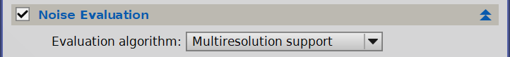
If this option is selected, ImageCalibration will compute per-channel estimates of the standard deviation of the noise and noise scaling factors for each target image, using a multiscale algorithm (the MRS noise estimator is used by default).
Noise estimates will be stored as a set of custom XISF properties and FITS header keywords in the output files. These estimates can be used later by several processes and scripts for specialized image analysis purposes, most notably by SubframeSelector and ImageIntegration for image grading and weighting.
The evaluation algorithm parameter allows selecting an algorithm for automatic estimation of the standard deviation of the noise in the calibrated images.
-
Multiresolution support (MRS)
-
The multiresolution support (MRS) noise estimation routine implements the iterative algorithm described by Jean–Luc Starck and Fionn Murtagh in their paper Automatic Noise Estimation from the Multiresolution Support.[9] In our implementation, the standard deviation of the noise is evaluated on the first four wavelet layers, assuming a Gaussian noise distribution. MRS is a remarkably accurate and robust algorithm and also the default option for noise evaluation.
-
Iterative k-sigma clipping
-
The iterative k-sigma clipping algorithm can be used as a last-resort option in cases where the MRS algorithm does not converge systematically. This can happen on images with no detectable small-scale noise, but should never happen with uncalibrated data under normal working conditions.
-
N* robust noise estimator
-
This noise estimator extracts a subset of residual pixels by comparison with a large-scale model of the local background of the image, generated with the multiscale median transform (MMT). Since the MMT is remarkably efficient at isolating image structures, it can be used to detect pixels that cannot contribute to significant structures. N* is an accurate and robust, alternative estimator of the standard deviation of the noise that does not assume or require any particular statistical distribution in the analyzed data.
Further information can be found in the Image Weighting Algorithms in PixInsight document, also available from the PixInsight core application in the Technical Documents section of the Resource main menu item.
Important— This option should always be enabled for calibration of non-CFA raw light frames, such as frames acquired with CCD and monochrome CMOS sensors. For CFA data, such as frames acquired with one-shot or DSLR color cameras, signal and noise evaluation should be performed by the Debayer process, and hence this option should be disabled in ImageCalibration in these cases.
2.6 Input Pedestal
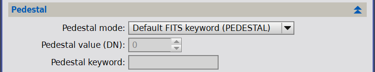
The same pedestal option is used for all input files (master and target frames). If you specify a pedestal, be sure that it can be the same for all your input files.
-
Pedestal mode
-
The pedestal mode option specifies how to retrieve a (usually small) quantity to be subtracted from input images as the very first calibration step. This quantity is known as pedestal, and must be expressed in the 16-bit unsigned integer range (from 0 to 65535). If present, a pedestal is assumed to be already added to the input data, either by the image acquisition software or by a previous calibration process, to ensure positivity of the result. For example, you might have specified an Output pedestal to enforce positivity of previously calibrated master bias, dark and flat frames.
-
Literal value
-
Allows to specify a pedestal value that will be subtracted from all target and master calibration frames. It is unlikely that a pedestal value is not otherwise specified, therefore this option is usually not needed, except in very special cases.
-
Default FITS keyword
-
This is the default mode. When this mode is selected, ImageCalibration will retrieve pedestal values from PEDESTAL FITS keywords, when they are present in the input images.
-
Custom FITS keyword
-
Allows you to specify the name of a custom FITS keyword to retrieve pedestal values, when the specified keyword is present in the input images.
Pedestal keyword values are always evaluated as their absolute values, that is, ignoring signs. This is because—another interoperability problem caused by the FITS format—some applications write PEDESTAL keywords to be added (negative) while others to be subtracted (positive). Ignoring the sign is safe in this case because all PEDESTAL values have (or should have) been added when they are present in FITS headers; therefore ImageCalibration simply subtracts their absolute values to get zero-based pixel data consistently.
-
-
Pedestal value (DN)
-
Literal pedestal value in the 16-bit unsigned integer range (from 0 to 65535), when the literal value option has been selected as pedestal mode.
-
Pedestal keyword
-
Custom FITS keyword to retrieve pedestal values in 16-bit DN. This is the name of a FITS keyword that will be used to retrieve input pedestals, if the custom FITS keyword option has been selected as pedestal mode.
2.7 Overscan
The overscan region of a CCD or CMOS, if present, is a part of the chip that is covered. Depending on the camera, it can be a useful way to remove small frame-to-frame variations in the bias level.
Each overscan allows you to define arbitrary source and target overscan regions in sensor pixel coordinates. You can define up to four overscan regions. Only the pixels parts of the final image region will be kept in the target image. The same overscan parameters are applied to all master frames with the Calibrate options and to the target frames (but each image is processed individually).
-
Image region
-
The image region defines a rectangular area of the raw frame that will be cropped after overscan correction. It usually corresponds to the true science image without any overscan regions. The four numeric values are expressed in pixels and refer to the leftmost column, topmost row, width and height of the image region of the sensor: at the end of the overscan correction procedure, the image will be cropped according to these values.
-
Source region
-
A source overscan region is used to compute an overscan correction value (as the median of all source region pixels) that will be subtracted from all pixels in the corresponding target region (see below). The four numeric values are expressed in pixels and refer to the leftmost column, topmost row, width and height of an overscan area of the sensor.
-
Target region
-
Defines the target region corresponding to the source region (see above). The four numeric values are expressed in pixels and refer to the leftmost column, topmost row, width and height of a target region of the sensor. Different target regions cannot overlap.
2.8 Master Bias
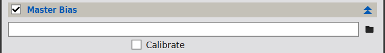
-
Master bias file
-
File path of the master bias frame.
-
If this checkbox is selected, ImageCalibration will calibrate the master bias frame at the beginning of the batch calibration process. Bias frames are only corrected for overscan, when one or more overscan regions have been defined and are enabled.
As a general rule, the master bias is only required when bias and dark data should be handled separately; for example, when dark frame optimization is applied, or when the bias signal is missing in the dark frames (i.e., when calibrated dark frames are used).
Note— As explained in the master calibration frames section, the use of calibrated master dark or bias is not recommended because this operation can lead to clipping of low data values and cause an incorrect noise evaluation.
2.9 Master Dark
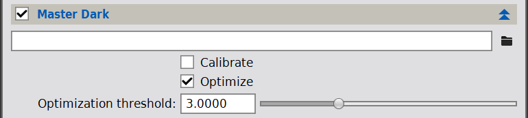
-
Master dark file
-
File path of the master dark frame.
-
Select this option to calibrate the master dark frame at the beginning of the batch calibration process. The master dark frame is corrected for overscan, when one or more overscan regions have been defined and are enabled, and bias-subtracted, if a master bias frame has been selected and is enabled.
-
Select this option to apply dark frame optimization.
The dark frame optimization routine computes a dark scaling factor to minimize the fixed pattern noise induced by dark subtraction. Optimization is carried out separately for each target frame, including the master flat frame, if selected and with its calibrate option active. Dark frame optimization has been implemented using multiscale (wavelet-based) noise evaluation and linear minimization routines.
-
Lower bound for the set of dark optimization pixels, measured in sigma units from the median.
This parameter defines the set of dark frame pixels that will be used to compute dark optimization factors adaptively. By restricting this set to relatively bright pixels, the optimization process can be more robust to readout noise present in the master bias and dark frames.
All pixels with a value below
 (where is the Optimization threshold and is the master dark) will be ignored by the noise evaluation routine during the dark frame optimization procedure. Increase this parameter to remove more dark pixels from the optimization set.
2.10 Master Flat
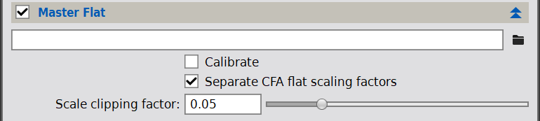
-
File path of the master flat frame.
-
Calibrate
-
Select this option to calibrate the master flat frame at the beginning of the batch calibration process. The master flat frame is corrected for overscan, bias-subtracted, and dark-subtracted with optional optimization, when the corresponding overscan regions and master calibration frames have been defined and are enabled.
-
When enabled and the master flat frame is a single-channel image mosaiced with a Color Filter Array (CFA), three separate master flat scaling factors are computed (see equation [8]).
This option helps when a strongly colored master flat frame is used, for example when a LED flat box with a strong blue component has been used to acquire flat frames. Computing different scaling factor prevents a strong color cast in the calibrated frames in these cases. When this option is disabled, a single scaling factor is computed for the whole master flat, ignoring CFA components.
-
Scale clipping factor
-
Master flat frame scaling factors are computed as robust mean pixel values for each channel or CFA component. This parameter defines the fraction of pixels that will be rejected to compute two-sided, symmetric trimmed means. The default value is 0.05, wich rejects a 5% of pixels at both ends of the flat frame distibution.
3 Usage
[hide]
Image calibration with the ImageCalibration tool is a straightforward process composed of several steps. ImageCalibration works together with the ImageIntegration tool to create master calibration frames.
The procedures described herewith are intended for common situations, and only the most important parameters are described: if not mentioned, a given parameter is considered to have its default value.
Although different approaches to calibration exist, our recommended practice is to use uncalibrated master dark frames that contain the bias signal, calibrated master flats and, if necessary, an uncalibrated master bias, for example when dark optimization is needed. The possible calibration of these master frames can be performed later (for example the overscan calibration).
Therefore the first calibration step is integrating individual dark frames, flat dark and bias frames into master frames using with the following settings.
-
Section Image Integration
-
- Combination: Average
- Normalization: No normalization
- Weights: Don't care (all weights = 1)
-
Section Pixel Rejection (1)
-
- Rejection algorithm: depends on the number of input frames; see the ImageIntegration documentation for recommendations. Usually the Winsorized Sigma Clipping algorithm is a good choice.
- Normalization: No normalization
-
Section Pixel Rejection (2)
-
The default values are usually good choices. Anyway, fine tuning is advisable to limit rejection to unwanted data, such as cosmic ray artifacts.
When the process is completed, the integration result, either the master dark or master bias, must be saved to disk for further calibration steps.
As explained in the master calibration frames section, we discourage the use of calibrated masters to avoid data clipping; that's why we integrate the bias and the dark frames directly without any calibration. Moreover, if the dark frame exposure time and temperature match the light frames, the bias frame is not required and can be ignored because its information is already present in dark frames.
3.1 Flat frame calibration
Flat field calibration consists in removing the additive signal coming from bias and dark current, so that only multiplicative information remains.
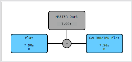
3.1.1 Calibration with flat dark
If a matching master flat dark is present the calibration procedure is very straightforward:
- Load the flat frames in the target frames list.
- Select an output directory where to save the calibrated flat frames.
- Disable the Signal Evaluation checkbox.
- Disable the Noise Evaluation checkbox.
- Disable the Master Bias section checkbox.
- Load the master flat dark as master dark.
- Disable both Calibrate and Optimize in the Master dark section.
- Disable the Master Flat section checkbox.
- Press the Apply global button

Calibration Diagram
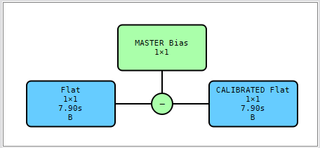
3.1.2 Calibration with bias
If a master flat dark is missing and the expected dark current is very low (typically with cooled cameras), flat frames can be calibrated with only a master bias obtained in the same conditions.
- Load the flat frames in the target frames list.
- Select an output directory where to save the calibrated flat frames.
- Disable the Signal Evaluation checkbox.
- Disable the Noise Evaluation checkbox.
- Load the master bias as master bias.
- Disable Calibrate in Master bias section.
- Disable the Master Dark section checkbox.
- Disable the Master Flat section checkbox.
- Press the Apply global button
Calibration Diagram
However, for sensors that exhibit "amplifier glow", the usage of dark frame optimization usually will not produce a correct calibration result. Therefore flat frames of sensors that exhibit "amp glow" should be calibrated using either only a master bias or, better, only a master flat dark, not applying dark frame optimization.
3.1.3 Calibration with an optimized master dark
If a master flat dark is missing, the flat frames can be calibrated with a master dark obtained with a different temperature and/or exposure time using the dark optimization feature.
Typically the flat frames are calibrated with the same master dark used for light frames. Under these conditions, to perform an excellent dark optimization routine, a master bias is necessary.
- Load the flat frames in the target frames list.
- Select an output directory where to save the calibrated flat frames.
- Disable the Signal Evaluation checkbox.
- Disable the Noise Evaluation checkbox.
- Load the master bias as master bias.
- Disable Calibrate in Master bias section.
- Load the master dark as master dark.
- Enable both Calibrate and Optimize in Master dark section.
- Disable the Master Flat section checkbox.
- Press the Apply global button
Calibration Diagram
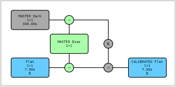
However, for sensors that exhibit "amplifier glow", the usage of dark frame optimization usually will not produce a correct calibration result. Therefore flat frames of sensors that exhibit "amp glow" should be calibrated using either only a master bias or, better, only a master flat dark, not applying dark frame optimization.
3.1.4 Integration of the calibrated flat frames
Finally, the calibrated flat frames must be integrated to generate the master flat frame using ImageIntegration with the following parameters:
-
Section Image Integration
-
- Combination: Average
- Normalization: Multiplicative
- Weights: Don't care (all weights = 1)
-
Section Pixel Rejection (1)
-
- Rejection algorithm: depends on the number of input frames; see the ImageIntegration documentation for recommendations. Usually the Winsorized Sigma Clipping algorithm is a good choice.
- Normalization: Equalize fluxes
-
Section Pixel Rejection (2)
-
The default values are usually good choices. Anyway, fine tuning is advisable to limit rejection to unwanted data, such as cosmic ray artifacts.
When the process is completed, the integration result, the master flat frame, must be saved to disk.
3.2 Light frame calibration
The light frame calibration procedure described herewith assumes that a full set of calibration masters is available. The recommended procedure is to use an uncalibrated master dark, a calibrated master flat and, if necessary, a master bias.
For monochrome cameras, the calibration must be done separately for each filter set. For OSC cameras, RAW non-demosaiced files should be used (even if ImageCalibration is actually able to work with RGB demosaiced images).
3.2.1 Calibration with a matching master dark
If an uncalibrated master dark frame with a matching exposure time and temperature is present, it also contains the bias signal. Therefore a master bias is not required.
- Load the light frames in the target frames list.
- Select an output directory where to save the calibrated light frames.
- If the images come from a one shot color camera (CFA images) Disable the Signal Evaluation checkbox.
- If the images come from a one shot color camera (CFA images) Disable the Noise Evaluation checkbox.
- Disable the Master Bias section checkbox.
- Load the uncalibrated master dark in Master Dark section.
- Disable both Calibrate and Optimize.
- Load the calibrated master flat.
- Disable Calibrate in Master flat section.
- If the light frames come from a One Shot Color (OSC) camera and the master flat was not demosaiced (as recommended), enable Separate CFA flat scaling factors. Disable this option if the images come from a monochrome camera.
- Press the Apply global button
Calibration Diagram

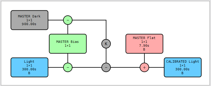
3.2.2 Calibration with an optimized master dark
If dark frame optimization shall be applied, a master bias is required. The master bias will be subtracted both from the light frames and the master dark, and a dark scaling factor k will be calculated for each light frame to minimize the variance after dark frame subtraction.
If a master dark with a matching exposure time and temperature is present, it also contains the bias signal. Therefore a master bias is not required.
- Load the light frames in the target frames list.
- Select an output directory where to save the calibrated light frames.
- If the images come from a one shot color camera (CFA images) Disable the Signal Evaluation checkbox.
- If the images come from a one shot color camera (CFA images) Disable the Noise Evaluation checkbox.
- Load the master bias in Master Bias section.
- Load the uncalibrated master dark in Master Dark section.
- Enable both Calibrate and Optimize.
- Load the calibrated master flat.
- Disable Calibrate in Master flat section.
- If the light frames come from a One Shot Color (OSC) camera and the master flat was not demosaiced (as recommended), enable Separate CFA flat scaling factors. Disable this option if the images come from a monochrome camera.
- Press the Apply global button
Calibration Diagram
3.3 Overscan calibration
The camera overscan region, if present, is a part of the sensor covered with an opaque coating. The overscan area can contain different kinds of information besides the "dark" signal. The horizontal register can be a bit longer than the width of the imaging area, so some overscan pixels may be only H-register pixels, not belonging to the actual image area. Actually, the overscan area can also contain some special-purpose pixels, like drain pixels. These additional pixels don't contain useful information for image processing and should not be included in the source area for overscan calibration; therefore the overscan source region in the Overscan section of ImageCalibration must be accurately defined.
Whether or not the overscan could be helpful depends on the camera. If the camera has a stable bias level, overscan calibration offers no benefits over traditional calibration. The bias stability can be assessed by taking a series of bias frames and measuring the average or the median level on each frame. This task can be accomplished, for example, with the BatchStatistics script.
The main goal of overscan calibration is to compensate for slight variations in the bias level from frame to frame. Overscan includes bias, read noise and dark current, but the dark current contribution is usually negligible and constant (if the temperature is controlled) and the read noise is significantly reduced by averaging all the pixels in the overscan source region.
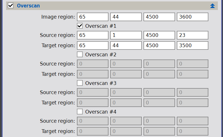
In the figure below we can see the structure of a KAF-16200 sensor.
In the figure above we can see that the overscan area contains many regions that should be ignored for overscan calibration. This figure gives us the necessary information to define the overscan image and source regions.
- The KAF-16200 is a single sensor with an imaging area of 4500×3600 pixels: this defines the size of the image region.
- The overscan area is composed of 65 columns to the left and 44 rows to the top, therefore the coordinates of the top left pixel of the image area are: x=65, y=44.
- The dark signal can be recovered from the frame around the active area. A suitable area could be, for example, a rectangle of 4500×23 pixels starting from x=65, y=1.
- Since the sensor is composed of a single CCD chip, the image and target regions are identical.
The recommended calibration workflow is to use an uncalibrated master dark, as explained at the beginning of this chapter, therefore the master dark still contains both the overscan information and the bias information.
The overscan area of each frame contains both the information on the bias offset and the dark current offset; therefore a master bias is usually not required. If, for some reason, you decide to use it, it should be uncalibrated.
When overscan data are defined ImageCalibration computes the median value of each source region and subtracts it to every single pixel in the corresponding target region. Then it crops the frame according to the image region. Overscan subtraction is applied to all the target frames and the master frames where the Calibrate option is enabled.
When calibrating mosaiced data (from OSC or DSLR cameras), pay special attention to the top left corner of the target overscan area. Defining incorrect origin coordinates may result in a wrong color filter array interpretation, and therefore in a wrong color rendition.
For a case study about overscan calibration read the Overscan Calibration in PixInsight article.
3.3.1 Flat frame calibration with overscan
As for the usual workflow, also in the calibration with overscan of the light frames, a calibrated master flat is recommended, therefore the single flat frames must be calibrated before integration.
The only differences from the usual workflow are:
- If a flat-dark frame is present, use it as a master dark, check the Calibrate checkbox, and uncheck the Optimize Checkbox.
- If a master dark frame with different exposure time is present, check both the Calibrate and Optimize checkboxes. A master bias is not required.
- If only a master bias frame is present, use it as a master bias, as usual, and check the Calibrate checkbox.
3.3.2 Light frame calibration with overscan
The recommended workflow needs only an uncalibrated master dark frame and a calibrated master flat frame.
The only differences from the usual workflow are:
- If a master dark with the same exposure time and temperature is present, check the Calibrate checkbox and uncheck the Optimize checkbox.
- If a master dark frame with a different exposure time is present, check both the Calibrate and Optimize checkboxes. A master bias is usually not required, even if, in a few cases, when the bias frame contains visible structures, it is a better practice to use it to completely separate the bias component from the time-dependent dark current.
3.4 How to verify dark frame optimization performance
As explained before, dark frame optimization is based on a few assumptions. The most important one is that it implicitly assumes that the dark optimization function is constant for the whole range of numerical data values and on the whole camera surface, since it consists of a single multiplicative factor. Unfortunately, this uniformity condition is not always true, so it is imperative to assess whether a camera is suitable for dark frame optimization or not. This task can be easily accomplished using ImageCalibration and ImageIntegration.
Here is the workflow to follow to make the test:
- Acquire a series of bias frames and integrate a master bias frame using ImageIntegration, as explained before.
- Acquire a series of dark frames with a long exposure time (for example, 600 seconds) and integrate a master dark frame using ImageIntegration, as explained before.
- Acquire a series of dark frames with a short exposure time (for example, 300 seconds).
- Using ImageCalibration, calibrate the short darks with the following steps:
- Load the short dark as target frames.
- Since after calibration a value close to zero is expected, in the Output Files section set a small Output Pedestal (for example, 1000 ADU should be enough) to avoid clipping.
- Load the master bias.
- Load the long master dark and enable both Calibrate and Optimize.
- Press the Apply global button
- Integrate the calibrated short dark frames with Imageintegration as for common dark frames.
- Apply a boosted automatic screen transfer function (STF) to the integrated image.
The integrated frame should appear almost perfectly flat, without structures and with only random noise scattered on the surface, if the optimization process worked as expected.
It is also important, during the calibration process, to pay attention to console messages where the dark scaling factor is shown for every calibrated file, like in the following sample:
Processing target frame: C:/Users/edoar/********
* Computing dark frame optimization factors.
Bracketing: done
Optimizing: done
* Performing image calibration.
* Performing noise evaluation.

* Writing output file: C:/Users/edoar/*******
Dark scaling factors:
k0 = 0.327
Gaussian noise estimates:
s0 = 1.049e-03, n0 = 0.917 (MRS)
Writing image: w=3474 h=2314 n=1 Gray Float32
29 FITS keyword(s) embedded.
8 image properties embedded.
The expected value is around the time ratio between the short and the long dark frame; for example, if the short dark frame exposure time is 300s and the long one is 600s, the expected value is around 0.500.
-
Example 1: CMOS with amplifier glow
-
The first example shows the optimization process on the dark frames from an old DSLR camera showing a strong amp glow.
- Temperature: Not controlled
- Long exposure time: 600 s
- Short exposure time: 300 s
- Expected = 1/2
Master dark and a calibrated dark frame with optimization:
In this case the optimization routine evaluates
 .
.As can be seen the amp glow is overcorrected and the dark scaling factor is much higher than expected: with this camera we cannot optimize dark frames correctly.
-
Example 2: CMOS without amplifier glow
-
The second example shows the optimization process on the dark frames from an DSLR camera (newer than the previous one) without obvious amp glow.
- Temperature: Not controlled
- long exposure time: 600 s
- short exposure time: 300 s
- Expected = 1/2
Master dark and a calibrated dark frame with optimization:
In this case the optimization routine evaluates
 .
.Observing the integration of the calibrated darks, it seems that the calibration result is much better than in the previous case, but the dark scaling factor has a completely unexpected value, so, in this case also, dark optimization is not recommended.
-
Example 3: Cooled CCD
-
The last example shows the optimization process on the dark frames from an CCD camera with active cooling.
- Temperature: -15°C
- Long exposure time: 900 s
- Short exposure time: 300 s
- Expected = 1/3
Master dark and a calibrated dark frame with optimization:
In this case the optimization routine evaluates
 .
.It is evident that the integration of the calibrated dark frames has a very good appearance, and the dark scaling factor has a value close to the expected value. With this camera the dark optimization feature will work flawlessly.

3.5 Calibration settings Summary
The following table summarizes the most common calibration settings.
Dark calibrated* |
Dark not calibrated |
|
|---|---|---|
Dark same temperature/time |
Bias frame: required Calibrate dark: OFF Optimize dark: OFF |
Bias frame: not required Calibrate dark: OFF Optimize dark: OFF |
Dark different temperature/time |
Bias frame: required Calibrate dark: OFF Optimize dark: ON* |
Bias frame: required Calibrate dark: ON Optimize dark: ON* |
Dark calibrated* |
Dark not calibrated |
|
|---|---|---|
Dark same temperature/time |
Bias frame: not required Calibrate dark: OFF Optimize dark: OFF |
Bias frame: not required Calibrate dark: OFF Optimize dark: OFF |
Dark different temperature/time |
Bias frame: not required Calibrate dark: OFF Optimize dark: ON* |
Bias frame: usually not required Calibrate dark: ON Optimize dark: ON* |
3.6 General settings for frame acquisition
3.6.1 Special recommendation for OSC cameras
When using an OSC camera (be it a regular digital camera or a dedicated astronomical camera), you generally want to perform the entire calibration process with raw CFA data. Raw CFA data are classified as 'Gray' in the 'Information' toolbar of PixInsight and are displayed as grayscale images. Only after the calibration process is completed (including if necessary) do the calibrated light frames have to be demosaiced to generate RGB color images. Subsequently, they are registered and finally integrated.
3.6.2 File formats
Using a regular digital camera that can save the data in a proprietary raw format (e.g., Canon's CR2 or CR3, Nikon's NEF, Sony's ARW or Fujifilm's RAF format), set your camera to use that raw format. Absolutely do not save data in JPEG or other formats using lossy compression schemes.
The acquisition software normally lets us choose whether the data from the camera will be saved to disk in the proprietary raw format, in FITS format, or both. The FITS format contains some useful metadata not stored in proprietary raw formats (such as the name and coordinates of the object, the focus position, etc.). Due to data compression, proprietary raw formats can generate smaller file sizes. Depending on the chosen file format, there is a difference in the data: the proprietary raw format contains intensity values in the bit depth of the analog-to-digital converter (ADC), e.g., for a 14-bit ADC in the range  . In contrast, the same data in a FITS file are scaled to 16 bit, i.e. they are multiplied by 4; hence the range is
  . Therefore using different file formats in the same project (light and calibration frames) may lead to severe issues in image calibration. So please follow the advice provided in the section Camera driver and acquisition software below. All the files must come in the same format.
3.6.3 Proprietary raw format of regular digital cameras
When camera data are saved to disk in a proprietary raw format, ascertain that the RAW Format Preferences in PixInsight (Format Explorer, double click on 'RAW') are set to Pure Raw. Nevertheless, by default, ImageCalibration uses the raw and CFA input hints that override the settings selected in the RAW module. The proprietary raw format contains the CFA mosaic pattern. When opening the file in PixInsight, the raw image decoding software used by PixInsight's RAW format support module (currently the LibRaw library) detects the CFA mosaic pattern and makes it available to the ImageCalibration and Debayer processes.
Since version 1.5.5, the RAW format support module has the new options Force focal length and Force aperture. When enabled, either no metadata will be generated for focal length and aperture, respectively (when the default value of 0 is left), or the specified values will be used. This is useful when the frames are captured with a telescope, where the camera cannot detect the correct values of focal length and aperture. In this case, the user should enable these options to avoid meaningless metadata (e.g., a default focal length of 50 mm).
3.6.4 FITS format
The camera driver or the acquisition software can provide image data in FITS format. As a general rule, the data are scaled to 16 bits (range 0 to 65535).
There are a few exceptions, though. Some Moravian camera models (e.g., the C2-12000A and presumably similar models) provide unscaled data. In these rare cases, the intensity values correspond to the bit depth of the ADC. So the C2-12000A, which utilizes the IMX304 sensor with a 12-bit ADC, provides data in the range from 0 to 4095.
The FITS header does not necessarily contain the CFA mosaic pattern for OSC cameras. Some acquisition software writes the non-standard FITS keywords 'BAYERPAT', 'XBAYROFF', 'YBAYROFF' and 'ROWORDER' supported by PixInsight ('ROWORDER' is new in PixInsight since version 1.8.8-6, see the mouse-over text in the FITS Format Preferences dialog). If the FITS keyword 'BAYERPAT' is not written to the FITS header, you must explicitly specify the correct CFA mosaic pattern (see the camera's handbook) when executing the ImageCalibration or the Debayer processes.
3.6.5 Camera driver and acquisition software
Some camera manufacturers provide two camera drivers: one 'native' driver and one ASCOM driver. To acquire frames for one project (light and calibration frames), always use the same camera driver, acquisition software, and file format. Different drivers, acquisition software, or file formats are not guaranteed to produce compatible results (e.g., scaling of intensity values or width and height of the frames). Such incompatibilities will invariably cause image calibration to produce wrong results or fail completely.
Using an OSC camera of ZWO, caution is advised when using the 'native' camera driver: the ZWO SDK enables the user in the acquisition software to control settings that influence the white balance of a displayed color image. Two parameters, WB_R and WB_B, achieve this with a data range from 1 to 100. The default values are WB_R = 52 and WB_B = 95. The intensities of the red channel will be multiplied by WB_R/50 and the intensities of the blue channel by WB_B/50. Unfortunately, the results of this multiplication are also written to disk in the FITS file. So it is important to set the values of both parameters to 50 and subsequently apply 'Save Config'; only in this way, the actual raw intensities will be saved to disk in the FITS files. Since camera data are usually saved in FITS files as signed 16-bit integers, rounding errors and clipping of high values will arise. Such a complication is generally avoided when the ASCOM camera driver is used instead of the native driver.
4 Credits
[hide]
This document was possible also thanks to the work of:
-
Jean-Marc Lugrin
-
Author of the original documentation regarding this tool; part of his job is still present in this official release.
-
Bernd Landmann
-
Author of the forum post Guide to Preprocessing of Raw Data with PixInsight, his job was a great inspiration for the structure and contents of this document.
References
[1] Wikipedia article: Photoelectric effect
[2] Wikipedia article: Salt-and-pepper noise
[3] Wikipedia article: Golden-section search
[4] Forum post: Jon Rista in QHY183M & Flats = Frustration, posts #57 and #63.
[5] Website: Abbas El Gamal, Stanford Engineering (2015), EE392B: Introduction to Image Sensors and Digital Cameras
[6] Website: KAF-16200 Datasheet. © Copyright 1999–2021 Semiconductor Components Industries, LLC
[7] Forum post: Juan Conejero, Dark Frame Optimization Algorithm
[8] Jean–Luc Starck and Fionn Murtagh (2002), Astronomical Image and Data Analysis, Springer-Verlag, pp. 37–38
[9] Jean–Luc Starck and Fionn Murtagh (1998). Automatic Noise Estimation from the Multiresolution Support. Publications of the Royal Astronomical Society of the Pacific, vol. 110, pp. 193–199
Copyright © 2023 Pleiades Astrophoto S.L.