1 Introduction
[hide]
Far better an approximate answer to the right question, which is often vague, than an exact answer to the wrong question, which can always be made precise.
The tool that is so dull that you cannot cut yourself on it is not likely to be sharp enough to be either useful or helpful.
— John Tukey
Modern astrophotography, based on digital cameras, is closely linked with the management and processing of digital images. In any digital image, the deterministic signal coming from the subject is affected by a measurement uncertainty due to the quantum nature of the light radiation: the noise. The weaker a subject is, the greater the degradation of its signal by the noise: the only way to improve the signal-to-noise ratio (SNR) of the image is to collect more signal; for example, by increasing the exposure time.
Unfortunately, the exposure time cannot be increased indefinitely. The solution is to break the single observation into numerous, shorter observations. During a typical astrophotography session, the photographer acquires many shots of the same subject, which will be combined later into a single image. Since the object's signal is deterministic but the noise is random, the effect of the combination is to reduce the noise, increasing SNR. This basic technique is called integration.
The simplest form of integration is a pixel-by-pixel arithmetic mean of a set  of images:
 [1]
[1]However, this equation can only generate an optimal result if all the images should have the same statistical weight, or in other words, if and only if all of the  images can contribute to the same extent to generate the best possible integrated image, according to some meaning of best.
Unfortunately, equation [1] is inadequate for real-world images: during an imaging session, varying conditions can continuously change image quality. Atmospheric extinction, seeing, air transparency, turbulence, thin clouds and tracking issues, are only a few possible sources of quality degradation. Therefore the single frames in an imaging campaign will likely have different qualities.
The solution to this problem is using a weighted combination formula, such as the weighted average of images:
 [2]
[2]Here the weight  represents a scalar quality funcion
  of
of  quality estimators
  ,
,  , for the
  image
image  in the set:
 [3]
[3]But what is exactly quality, and how can we measure it? The concept of image quality is not straightforward by any means: the signal-to-noise ratio can be used as a quality measure, but it is not the only possibility. For example, quality can be having rounder stars, or a more intense signal, or more resolution, or a greater number of detectable stars, or any arbitrary combination of all of these factors, and more, which is found to be optimal for a specific purpose.
Here we reach the main subject of this article. In version 1.8.9 of PixInsight we have introduced a new class of photometry-based image quality estimators and weighting algorithms, which we are going to describe in the following sections. These algorithms are tightly integrated with our standard data reduction and image preprocessing pipeline, from image calibration to image integration and drizzle integration. We'll describe the algorithms technically, and then will provide extense information on their current implementation in the tools and processes involved. We'll complete the document with some interesting examples and a special section on a linear regression analysis of the algorithms, contributed by John Pane.
2 PSF Flux Weighting Algorithms
[hide]
PSF Signal Weight (PSFSW) is a new image quality estimation algorithm based on a hybrid PSF/aperture photometry measurement methodology. PSFSW has been designed to be a robust, comprehensive estimator able to capture a number of critical image quality variables into a single scalar function. PSF SNR is a realization of the ratio of powers paradigm for signal-to-noise ratio evaluation, also based on the same measurement techniques. We outline the operational components of these algorithms in the following subsections.
2.1 PSF Fitting
We begin by detecting a set of sources in the image. This first step is critical because we want to detect stars, not extended objects or potential bright artifacts such as uncorrected hot pixels, cosmic ray impacts, satellite and plane trail residuals, etc. We already have this task well implemented in our code base and have been improving it for many years. The second step is fitting a point spread function (PSF) to each detected star. Our implementation of PSF fitting is based on the Levenberg-Marquardt[1] algorithm and has also been part of our code base for a long time. We have improved substantially these fitting routines in recent versions of PixInsight. Our current implementation supports elliptical Gaussian and Moffat[2] functions for PSF flux evaluation. These functions are given by
 [4]
[4]and
 [5]
[5]respectively, where the parameters are:
-

-
Average local background.
-

-
Amplitude, which is the maximum value of the fitted PSF, and also the function's value at the centroid coordinates.
-

-
Centroid coordinates in pixel units. This is the position of the center of symmetry of the fitted PSF.
-

-
Standard deviations of the PSF distribution on the horizontal and vertical axes, measured in pixels. Conventionally, the X axis corresponds to the direction of the semi-major axis of the fitted elliptical function.
-

-
Moffat shape parameter.

Figure 1 — Some point spread function profiles. The full width at half maximum (FWHM) and full width at tenth maximum (FWTM) are standard measures to quantify the dimensions of a fitted PSF.
2.1.1 Rotated Functions
When the difference between  and
and  is larger than the nominal fitting resolution (0.01 pixel in the current implementation), our PSF fitting routines fit an additional
  parameter, which is the rotation angle of the X axis with respect to the centroid position. varies in the range [0°,180°). For a rotated PSF, the
  and
and  coordinates in the above equations must be replaced by their rotated counterparts
  and
and  respectively:
 [6]
[6]2.1.2 Adaptive Sampling Region
Each PSF is fitted from pixels inside a square sampling region centered at the approximate central coordinates of the detected source. The size of each sampling region is determined adaptively by a median stabilization algorithm. Basically, the sampling region starts at the limits of the detected source structure and grows iteratively until no significant change is detected in the median calculated from all pixels within the region. This improves accuracy and resilience to outliers in fitted local background estimates, which are crucial for the accuracy of fitted PSF models and hence of PSF flux estimates.
2.1.3 Automatic PSF Type Selection
Our current implementation supports an automatic mode for selection of an optimal PSF type for each detected source. When this mode is selected, a series of different PSFs will be fitted for each source, and the fit that leads to the least absolute difference among function values and sampled pixel values will be used for flux measurement. Currently the following functions are tested in this special automatic mode: Moffat functions with shape parameters equal to 2.5, 4, 6 and 10. This limited set represents a compromise between accuracy and efficiency with current computational resources. We will be adding more sophistication to this adaptive PSF type selection strategy in future versions.

2.2 PSF Flux Evaluation
Once we have a set of detected sources with their corresponding fitted point spread functions, we compute a PSF flux estimate for each source:
 [7]
[7]where  is the elliptical measurement region, defined by default at the one tenth maximum level (FWTM) of the fitted PSF,
  represents a set of image coordinates within ,
  is the pixel sample value at , and
  is the fitted local background estimate.
We define also the mean PSF flux estimate:
 [8]
[8]with the semimajor axes of the measurement region given by
 [9]
[9]and
 [10]
[10]where  is a growing factor parameter (
 by default). Using the area of the elliptical measurement region calculated from fitted PSF parameters gives more accurate results than the number of sampled pixels for mean PSF flux estimates, especially for undersampled images and small sources in general.
Note that fitted (amplitude) parameters are not used for PSF flux evaluation, since flux is calculated exclusively from sampled image pixels. This leads to our hybrid PSF/aperture photometry approach.
2.2.1 Outlier Rejection
In general, the set of PSF flux estimates obtained from sources detected in a calibrated raw frame, where low SNR is always an important conditioning factor, tends to show large dispersion and contain a significant fraction of outliers. Rejecting wrong measurements is thus imperative to achieve consistent results in our quality estimator. We have implemented ideas and algorithms from the Robust Chauvenet Outlier Rejection paper by M. P. Maples et al. (2018)[7], which have proven to perform remarkably well to achieve clean sets of PSF flux measurements, even under very low SNR and difficult star detection conditions.
2.3 Robust Mean Background Estimator
The next component of the PSFSW algorithm is a robust estimate of mean background. This estimate allows us to characterize the mean large-scale illumination level of each subframe in a data set, thus making PSFSW sensitive to background gradients, which are important variables for quality estimation.
We represent the multiscale median transform (MMT)[3] as
 [11]
[11]with multiscale levels (or layers), scaling distance  , and
, and  the image being evaluated. MMT is a nonlinear transform that generates an ordered list of multiscale levels
  , which isolate image structures at growing dimensional scales by the application of median filters of increasing sizes. Each level is a matrix with the same dimensions as the transformed image, so the MMT is redundant. Each level contains difference transform coefficients between two successive scales, so the inverse transform is the sum of all transform levels. The last level
  is the large-scale residual level, which is the only one in which we are interested here; the rest of detail levels are successively evaluated but discarded for this application.
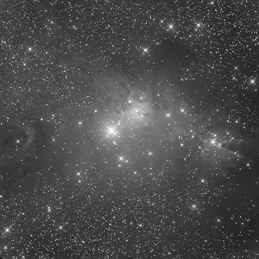
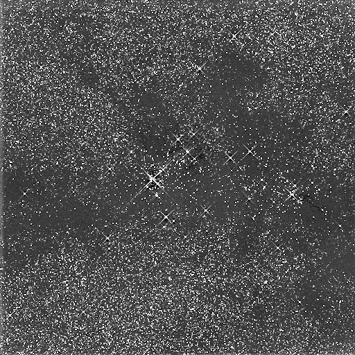
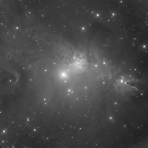


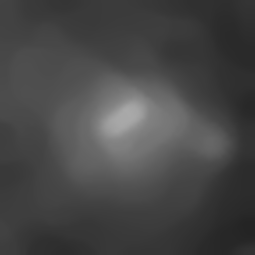
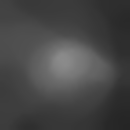
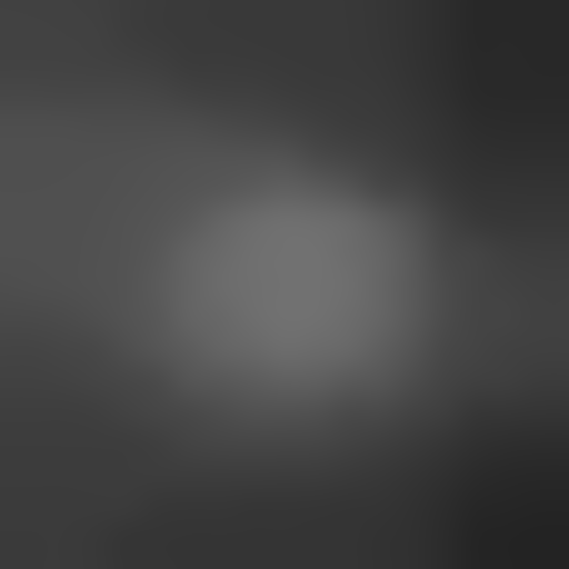
Figure 4 — Multiscale Median Transform residuals. From top to bottom, left to right: The original image, the first MMT level at the scale of one pixel, and residual levels at the scales of 32, 64, 128, 256, 512, 1024 and 2048 pixels, respectively.
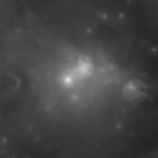

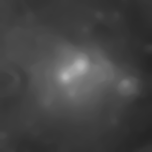
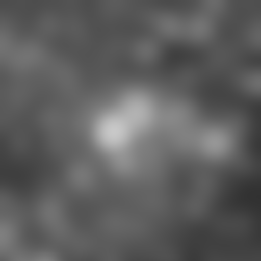
Figure 5 — Comparison between the multiscale median transform (MMT) and the starlet transform (ST, also known as à trous wavelet transform) for structure isolation with the same image used in Figure 4. Linear multiscale transforms such as ST cannot isolate small-scale bright structures, such as stars, within a reduced set of small-scale levels.
Top row: residual MMT and ST levels at the scale of 128 pixels.
Bottom row: residual MMT and ST levels at the scale of 256 pixels.
In linear multiscale transforms stars pervade the entire transform, contaminating all levels, even at very large scales. This makes linear transforms useless to generate models representative of the image at such large scales, while nonlinear transforms such as MMT are remarkably efficient at this task.
Define the MMT residual as the set:
 [12]
[12]The  set gathers all pixels with values smaller than a large-scale local background model generated with the MMT. No pixel in can belong to significant image structures as represented by the applied MMT. In the current implementation these local background models are generated at the scale of 256 pixels by default.

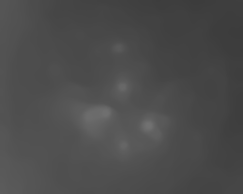
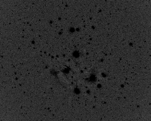
Figure 6 — Top left: original image.
Top right: MMT local background model at the scale of 256 pixels.
Bottom left: MMT residual.
Now define our robust mean background estimator as:
 [13]
[13]This solution works remarkably well thanks to the efficiency of MMT to isolate image structures. The  background estimate effectively isolates all non-significant pixels and is immune to irregular illumination variations, since all pixels are evaluated against a local background model of the image.
2.4 Robust Noise Estimators
The multiresolution support noise evaluation algorithm (MRS)[4] is currently the standard noise estimator in PixInsight. This algorithm uses the starlet transform[3] (aka à trous wavelet transform) to estimate the standard deviation of the noise, assuming a Gaussian noise distribution, with variations to support mixed Gaussian/Poisson distributions. Succinctly, the MRS algorithm classifies pixels by their belonging to two disjoint sets of significant and non-significant image structures using a data structure known as multiresolution support. The standard deviation of all pixels not belonging to significant structures is the noise estimate. The MRS algorithm is remarkably robust and accurate, and provides estimates accurate to within a 1% in most cases. Refer to the references for a detailed description.
In deriving the robust mean background estimator we get an additional noise estimator, which we define in two variants:
 [14]
[14]and
 [15]
[15]where we use either the median absolute deviation from the median (MAD) or the  scale estimator of Rousseeuw and Croux[5]. The normalization constants are necessary to make these noise estimators consistent with the standard deviation of a Gaussian distribution. We have found these constants for our current implementation by running a bootstrap estimation[6] with 10,000 synthetic 16 megapixel, Gaussian white noise images.
Figure 7 — A script for bootstrap estimation of the efficiency and normalization factors of a scale estimator with respect to the standard deviation of a normal distribution. Warning: As it is configured below, running this script may require a long time, from a few hours to several days, depending on hardware performance. For quick tests you can redefine the numberOfSamples macro with a small number of images, such 5 or 10.
#include <pjsr/UndoFlag.jsh>

#define sampleSize      4096
#define numberOfSamples 10000

function bootstrap( estimator )
{
   console.show();
   console.writeln( "<end><cbr>Performing bootstrap, please wait..." );
   console.flush();

   let P = new PixelMath;
   P.expression = "gauss()";
   P.rescale = true;
   P.truncate = false;

   let window = new ImageWindow( sampleSize, sampleSize, 1, 32/*bps*/, true/*float*/, false/*color*/ );
   let view = window.mainView;
   view.beginProcess( UndoFlag_NoSwapFile );
   let image = view.image;

   let R = new Float32Array( numberOfSamples );
   let S = new Float32Array( numberOfSamples );
   let K = new Float32Array( numberOfSamples );

   let T = new ElapsedTime;

   for ( let i = 0; i < numberOfSamples; ++i )
   {
      P.executeOn( view, false/*swapFile*/ );
      processEvents();
      let r = image.stdDev();
      let s = estimator( image );
      R[i] = r;
      S[i] = s;
      K[i] = r/s;
   }

   let k = Math.median( K );
   for ( let i = 0; i < numberOfSamples; ++i )
      S[i] *= k;
   let var_r = Math.variance( R );
   let var_s = Math.variance( S );

   view.endProcess();
   window.forceClose();

   console.writeln( format( "<end><cbr><br>Variance of stddev ...... %.4e", var_r ) );
   console.writeln( format(               "Variance of estimator ... %.4e", var_s ) );
   console.writeln( format(               "Gaussian efficiency ..... %.3f", var_r/var_s ) );
   console.writeln( format(               "Normalization factor .... %.5f", k ) );
   console.writeln( T.text );
}

/*
 * N* noise estimator - MAD variant
 */
function NStar_MAD( image )
{
   return Math.MAD( image.mmtBackgroundResidual( 256 ) );
}

/*
 * N* noise estimator - Sn variant
 */
function NStar_Sn( image )
{
   return Math.Sn( image.mmtBackgroundResidual( 256 ) );
}

bootstrap( NStar_Sn );
Despite the fact that the MRS and  algorithms generally produce similar values for most astronomical images, these estimators are very different. MRS usually evaluates a relatively small fraction of pixels on dark background areas, where the noise completely dominates the distribution of pixel values on the whole image. , on the other hand, tends to evaluate approximately one half of the available pixels on average, since it estimates the dispersion of the MMT residual below a local background model. This means that is a relative noise evaluation algorithm. Put in simpler words, if we for example evaluate for an image with large free background areas and then for a small crop dominated by bright structures, we'll in general obtain different results. is a comprehensive noise estimator able to evaluate the uncertainty in the data irrespective of local intensity levels. However, this estimator must only be used to compare noise estimates calculated for similar images, such as those in a data set acquired consistently for the same region of the sky. It should also be noted that does not assume or require any particular statistical distribution in the analyzed image.
2.5 The PSF Signal Weight Estimator of Image Quality
We now have all of the necessary elements to build our PSFSW estimator, which we define as:
 [16]
[16]where  is a noise estimate, which can be calculated with either the MRS or the algorithm (MRS is used by default), and
  are normalization constants.
In this equation, the sum of PSF flux estimates provides a measurement of the total signal in the evaluated image. Obviously, more signal means a stronger image. The sum of mean PSF flux estimates, on the other hand, is a measure of signal concentration. In other words, the mean PSF fluxes introduce a dependency on the average size of the stars in the PSFSW equation: the higher the sum of mean flux estimates, the higher the resolution of the evaluated image. Looking at the denominator of the equation we find a noise estimate, which plays the role of error measurement, multiplied by our robust mean background estimate, which accounts for relative background variations caused by light pollution gradients, passing clouds, poor transparency, moonlight and similar effects.
The normalization constants have been determined to provide manageable typical estimates in the range from 0.01 to 100 for most deep-sky images. To find these constants we have performed a simulation with 1000 synthetic linear images generated under controlled conditions:
- Image dimensions: 4096 × 4096 pixels.
- Background: synthetic Gaussian noise with standard deviation = 0.001 and mean = 0.015.
- Star field: 1500 detectable stars per image on average, Moffat PSF with β=4 and FWHM = 5 pixels.
- Noise: Combined synthetic Poisson noise and Gaussian white noise with the standard deviation of the image.
The 1000 simulated images were used to compute PSFSW estimates with default parameters, and the normalization constants were adjusted for this set to achieve unit median PSFSW:
 [17]
[17]

2.6 The PSF SNR Robust Estimator of Signal-To-Noise Ratio
The PSF SNR estimator is a realization of the signal-to-noise ratio formulation based on the ratio of powers paradigm:
 [18]
[18]Used directly for image weighting, this estimator is a good option when one wants to maximize SNR exclusively in the integrated image, disregarding other quality variables. The normalization factors were derived from the same simulated data set used for calibration of PSFSW. In this case we adjusted the coefficients to achieve equal median values for PSF SNR and the standard SNR estimator:
 [19]
[19]which leads to  for the simulated data set.
2.7 The SNR Estimator
For completeness and consistency of comparisons, we'll describe also our standard SNR estimator based on global estimates of scale instead of stellar photometry. The SNR estimator is defined as
 [20]
[20]where  is a scale estimate calculated for the image and is, as before, an estimate of the standard deviation of the noise. This corresponds to the ratio of powers standard formulation of signal-to-noise ratio.
SNR allows us to implement a scaled version of the inverse variance weighting method.[8] When SNR estimates are used to compute a weighted average of a set of images (considered here as a set of independent observations), the resulting average works as a maximum likelihood estimator of deterministic signal. This means that SNR weights are theoretically optimal in terms of SNR maximization.
The standard deviation of the noise can be evaluated without problems with one of the algorithms that we have already implemented, such as the MRS algorithm, which is remarkably robust. However, a meaningful estimate of dispersion for the image is problematic in this context because we need a highly efficient estimator, which excludes robust scale estimators. This is an excellent example of the robustness versus efficiency problem in statistics. Basically, no (known) estimator of statistical scale works for this task except the standard deviation. The reason is that any attempt to reject outliers beyond a delicate limit damages the efficiency of the estimator, which leads to a meaningless result. In our current implementation we have designed a special method to evaluate the standard deviation of the image in three successive iterations, rejecting pixels with decreasing tolerances based on the previous estimates. This is a sort of self-stabilizing estimator that performs a slight but sufficient rejection of outliers without damaging efficiency. In addition, the estimator is bilateral, which means that variability is evaluated separately for pixels below and above the median. This makes it even more efficient for asymmetrical distributions. Despite these efforts, SNR is sensitive to large outliers, such as airplane trails and similar artifacts, which inevitably degrade its performance to extents proportional to the amount of outlier pixels. A representative example of this is shown in Figure 9.
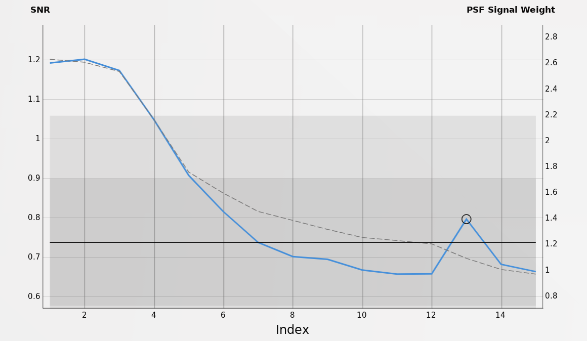
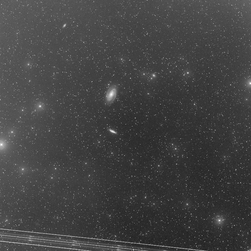
Figure 9 — A SubframeSelector graph showing a typical robustness issue with the SNR estimator for a set of wide field images of the M81/M82 region (Finger Lakes ProLine PL16801 CCD camera, blue filter). The frame at index 13, shown above and indicated with a circle on the graph, has a big airplane trail that introduces a strong bias in the variance used as the numerator of the SNR equation (see Equation [20]). Neither PSFSW nor PSF SNR have these problems. In this example, note that PSFSW is plotted in the graph along with SNR, showing it is resistant to the airplane trail in frame #13.
As the basis of a maximum likelihood estimator, SNR is very useful as a reference for counter-tests and comparisons with other quality metrics. This is true despite the robustness problems that we have described, and one of the reasons why we preserve SNR among the main properties available for weights and graphs in the SubframeSelector tool.
A different class of problems associated with the use of SNR for image weighting comes from its inability to react against background gradients as one would expect from a quality estimator. The problem here is not that SNR is wrong, as we have read so many times, but rather that SNR is neither an image quality estimator nor a selective SNR estimator working with high-signal image structures (as PSF SNR does for example). SNR evaluates global properties of the image, and it does that well, although it may not give the expected results if used to answer the wrong questions. We'll see this better in the examples included later in this document.
3 Implementation
[hide]
In this section we describe the current implementation of the new image weighting algorithms in several important processes of our standard data reduction and image preprocessing pipeline. We describe the relevant parameters available in several tools and provide practical usage information.
It is important to point out that the actual image weights are not stored in the images generated by any of the tools in our preprocessing pipeline. All of these tools generate and/or use specific metadata to compute the weights when necessary. At the end of this section we describe also the metadata currently generated for the application of these algorithms.
3.1 ImageCalibration and Debayer
The ImageCalibration and Debayer tools have two new sections since version 1.8.9 of PixInsight, namely Signal Evaluation and Noise Evaluation, which provide most of the necessary parameters to control the new PSF flux based image weighting algorithms.
Important— It cannot be overemphasized that signal and noise evaluation must be carried out by different processes, depending on the type of raw data:
- Monochrome CCD or CMOS raw frames: signal and noise evaluation must be performed by the ImageCalibration process.
- Mosaiced CFA raw frames: signal and noise evaluation must be performed by the Debayer process. Debayer will always compute noise estimates before demosaicing, that is, from uninterpolated raw calibrated data.
If you use our standard WeightedBatchPreprocessing script to calibrate your data, and to demosaic it when appropriate, then the correct procedures will always be applied.
3.1.1 Signal Evaluation
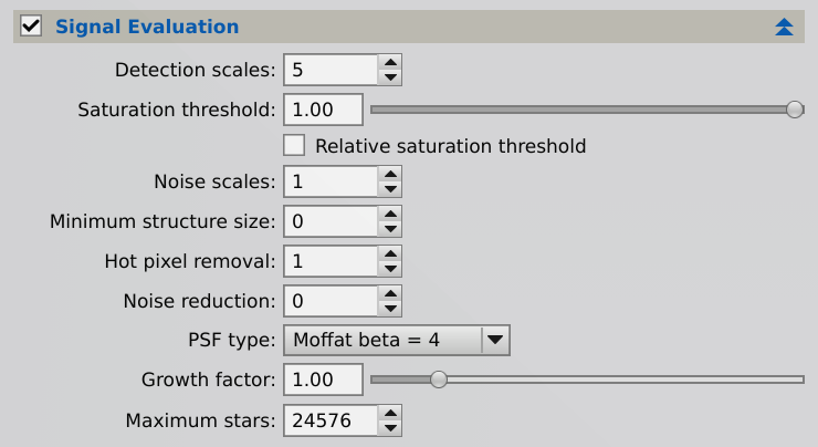
Many of the parameters in this section provide control over the initial star detection phase. In most cases there is no need to change the values of these parameters, since our star detection routines are robust even under quite unfavorable conditions. However, in particularly problematic cases the availability of these parameters can become very useful.
-
Detection scales
-
Our star detection routines implement a multiscale algorithm. This is the number of wavelet layers used for structure detection. With more wavelet layers, larger stars, but perhaps also some nonstellar objects, will be detected.
-
Saturation threshold
-
Detected stars with one or more pixels with values above this threshold will be excluded for signal evaluation. This parameter is expressed in the [0,1] range. It can be applied either as an absolute pixel sample value in the normalized [0,1] range, or as a value relative to the maximum pixel sample value of the measured image (see the Relative saturation threshold parameter below).
The default saturation threshold is 1.0. For signal evaluation, the implemented star detection and outlier rejection routines are normally able to avoid contamination from saturated sources, so the default value of this parameter should not be changed under normal conditions.
-
Relative saturation threshold
-
The saturation threshold parameter, when it is set to a value less than one, can be applied either as an absolute pixel sample value in the normalized [0,1] range, or as a value relative to the maximum pixel sample value of the measured image. The relative saturation threshold option is enabled by default.
-
Noise scales
-
Number of wavelet layers used for noise reduction. Noise reduction prevents detection of bright noise structures as false stars, including hot pixels and cosmic rays. This parameter can also be used to control the sizes of the smallest detected stars (increase it to exclude more stars), although the minimum structure size parameter can be more efficient for this purpose.
-
Minimum structure size
-
Minimum size of a detectable star structure in square pixels. This parameter can be used to prevent detection of small and bright image artifacts as stars, when such artifacts cannot be removed with a median filter (i.e., with the hot pixel removal parameter).
Changing the default zero value of this parameter should not be necessary with correctly acquired and calibrated data. It may help, however, when working with poor quality data such as poorly tracked, poorly focused, wrongly calibrated, low-SNR raw frames, for which our star detection algorithms have not been designed specifically.
-
Hot pixel removal
-
Size of the hot pixel removal filter. This is the radius in pixels of a median filter applied by the star detector before the structure detection phase. A median filter is very efficient to remove hot pixels. If not removed, hot pixels will be identified as stars, and if present in large amounts, can prevent a valid signal evaluation. To disable hot pixel removal, set this parameter to zero.
-
Noise reduction
-
Size of the noise reduction filter. This is the radius in pixels of a Gaussian convolution filter applied to the working image used for star detection. Use it only for very low SNR images, where the star detector cannot find reliable stars with its default parameters. To disable noise reduction, set this parameter to zero.
-
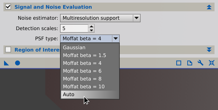
PSF type
-
Point spread function type used for PSF fitting and photometry. In all cases elliptical functions are fitted to detected star structures, and PSF sampling regions are defined adaptively using a median stabilization algorithm.
When the Auto option is selected, a series of different PSFs will be fitted for each source, and the fit that leads to the least absolute difference among function values and sampled pixel values will be used for flux measurement. Currently the following functions are tested in this special automatic mode: Moffat functions with β shape parameters equal to 2.5, 4, 6 and 10.
The rest of options select a fixed PSF type for all detected sources, which improves execution times at the cost of a less adaptive, and hence potentially less accurate, signal estimation process.
-
Growth factor
-
Growing factor for expansion/contraction of the PSF flux measurement region for each source, in units of the Full Width at Tenth Maximum (FWTM).
The default value of this parameter is 1.0, meaning that flux is measured exclusively for pixels within the elliptical region defined at one tenth of the fitted PSF maximum. Increasing this parameter can improve accuracy of PSF flux measurements for undersampled images, where PSF fitting uncertainty is relatively large. Decreasing it can be beneficial in some cases working with very noisy data to restrict flux evaluation to star cores.
-
Maximum stars
-
The maximum number of stars that can be measured to compute PSF flux estimates. PSF photometry will be performed for no more than the specified number of stars. The subset of measured stars will always start at the beginning of the set of detected stars, sorted by brightness in descending order.
The default value imposes a generous limit of 24K stars. Limiting the number of photometric samples can improve performance for calibration of wide-field frames, where the number of detected stars can be very large. However, reducing the set of measured sources too much will damage the accuracy of signal estimation.
3.1.2 Noise Evaluation
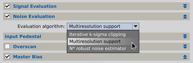
This section allows you to control the noise evaluation algorithm used for generation of PSF flux based metadata, which in turn is used in the calculation of PSF Signal Weight and PSF SNR estimates.
-
Evaluation algorithm
-
This option selects an algorithm for automatic estimation of the standard deviation of the noise in the calibrated/demosaiced images.
The multiresolution support (MRS) noise estimation routine implements the iterative algorithm described by Jean-Luc Starck and Fionn Murtagh in their 1998 paper Automatic Noise Estimation from the Multiresolution Support.[4] In our implementation, the standard deviation of the noise is evaluated on the first four wavelet layers, assuming a Gaussian noise distribution. MRS is a remarkably accurate and robust algorithm and the default option for noise evaluation.
The iterative k-sigma clipping algorithm can be used as a last-resort option in cases where the MRS algorithm does not converge systematically. This can happen on images with no detectable small-scale noise, but should never happen with raw or calibrated data under normal working conditions, so this option is available more for completeness than for practical reasons.
The N* robust noise estimator extracts a subset of residual pixels by comparison with a large-scale model of the local background of the image, generated with the multiscale median transform (MMT). Since the MMT is remarkably efficient at isolating image structures, it can be used to detect pixels that cannot contribute to significant structures. N* is an accurate and robust, alternative estimator of the standard deviation of the noise that does not assume or require any particular statistical distribution in the analyzed data.
3.2 SubframeSelector
The SubframeSelector tool was written by Cameron Leger in 2017, based on the homonym script written by Mike Schuster, back in 2013. Both PTeam members made fundamental contributions to the PixInsight platform with this powerful image analysis infrastructure of unparalleled efficiency and versatility. Since the initial release of the SubframeSelector tool we have been improving it at a constant rate to incorporate new advances in image analysis developed on the PixInsight platform. Obviously, development of the new image quality estimators subject of the present article is no exception. Since version 1.8.9 of PixInsight, the new PSF Signal Weight and PSF SNR estimators are tightly integrated with our standard preprocessing pipeline, including the SubframeSelector tool as an essential actor.
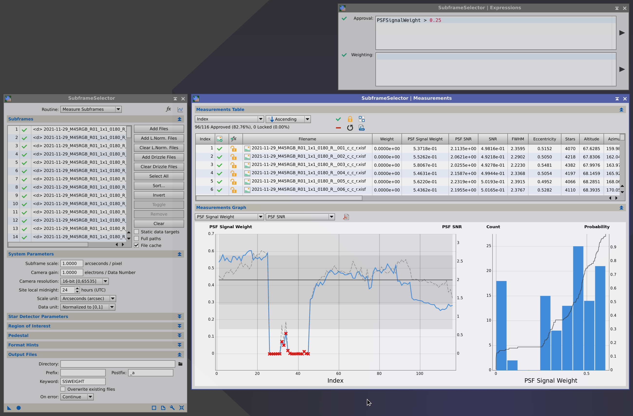
The SubframeSelector tool supports a new set of variables (also called properties) for image selection and weighting, as well as for subframe sorting and graph generation. Refer to the reference documentation of this tool for complete information. The following list includes all supported variables for completeness of reference. In all cases the value of each variable is computed separately for each measured subframe.
-
Altitude
-
The altitude above the horizon for the equatorial coordinates of the center of the subframe at the time of acquisition, in the range [0°,+90°].
-
Azimuth
-
The azimuth for the equatorial coordinates of the center of the subframe at the time of acquisition, in the range [0°,360°).
-
Eccentricity
-
A robust mean of the set of measured eccentricities from all fitted PSFs.
-
EccentricityMeanDev
-
The mean absolute deviation from the median of the set of Eccentricity values.
-
FWHM
-
A robust mean of the set of full width at half maximum (FWHM) measurements for all fitted PSFs.
-
FWHMMeanDev
-
The mean absolute deviation from the median of the set of FWHM values.
-
Index
-
The one-based index of the subframe, in the [1,n] range, where n is the number of measured subframes.
-
Median
-
The median pixel sample value.
-
MedianMeanDev
-
The mean absolute deviation from the median.
-
MStar
-
The
robust mean background estimate. -
Noise
-
The noise estimate. This is the MRS estimate by default, unless a different option has been selected in the ImageCalibration or Debayer tools.
-
NoiseRatio
-
The fraction of pixels used for noise evaluation with the MRS algorithm, in the [0,1] range. Always zero when the
algorithm is used to compute noise estimates. -
NStar
-
The
robust noise estimate. -
PSFCount
-
The number of PSF fits used for PSF flux evaluation.
-
PSFFlux
-
The sum of all PSF flux estimates.
-
PSFFluxPower
-
The sum of all PSF squared flux estimates. Currently not used, reserved for future extensions.
-
PSFSignalWeight
-
The PSF Signal Weight (PSFSW) estimate of image quality.
-
PSFSNR
-
The PSF SNR estimate.
-
PSFTotalMeanFlux
-
The sum of all PSF mean flux estimates.
-
PSFTotalMeanPowerFlux
-
The sum of all PSF mean squared flux estimates. Currently not used, reserved for future extensions.
-
SNR
-
The SNR estimate.
-
SNRWeight
-
An alias for the SNR estimate, for backward compatibility.
-
StarResidual
-
A robust mean of the set of MAD estimates for all fitted PSFs. Each MAD estimate is a Winsorized mean absolute deviation of fitted function values with respect to pixel values measured on the PSF sampling region.
-
StarResidualMeanDev
-
The mean absolute deviation from the median for the set of StarResidual values.
-
Stars
-
The total number of sources detected and fitted by the star detection and PSF fitting routines integrated in the SubframeSelector tool.
Each variable (excluding Index) also has a Median, Min and Max version (e.g. FWHMMin), which are computed across all subframes. Each variable (excluding Index) also has a Sigma version (e.g. PSFSignalSigma), where the value is expressed in sigma units of the mean absolute deviation from the median.
Important— SubframeSelector expects all signal and noise evaluation metadata items to be present in its input subframes. This can only happen if the subframes have been calibrated, and demosaiced when appropriate, with current versions of our ImageCalibration and Debayer tools. When signal and/or noise evaluation metadata items are not available for a subframe, the SubframeSelector tool computes them directly from input subframe pixels. In such case, if the subframe has been interpolated in some way (for example, after demosaicing and/or image registration), the computed items can be inaccurate (especially noise estimates) and hence the derived PSFSW and PSF SNR values can also be inaccurate, or even wrong in extreme cases. Appropriate warning messages are shown when this happens.
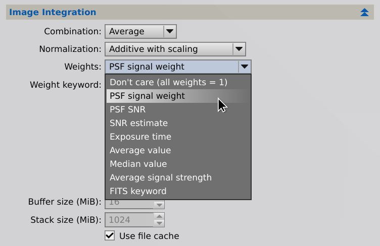
3.3 ImageIntegration and DrizzleIntegration
Since version 1.8.9 of PixInsight our standard ImageIntegration tool supports the new PSF Signal Weight (PSFSW) and PSF SNR estimators for calculation of image weights. The weighted average combination of images can be represented by the equation
 [21]
[21]for each non-rejected pixel at  coordinates, where is the weight assigned to the image
  As we have explained in the introduction of this document, different weights can be assigned to maximize (or minimize) different properties of the integrated image. When the PSFSW estimator is selected for weighting, the integration is optimized for a balanced set of image quality variables, including metrics representing SNR and image resolution; the ability of PSFSW to capture important quality metrics will be analyzed in the Linear Regression Analysis section. When the PSF SNR estimator is used, the integration tends to be optimized for maximization of SNR in the integrated result.
As an option, which is enabled by default, the ImageIntegration process can perform signal and noise evaluations for the integrated image, generating the same metadata as the ImageCalibration and Debayer processes. Currently the ImageIntegration tool provides a reduced set of parameters to control these evaluations; the rest of parameters governing these algorithms are left with default values.
As for the DrizzleIntegration process, ImageIntegration will include image weights in updated .xdrz files, which DrizzleIntegration will apply to its input images to generate a weighted, drizzle integrated image.
Important— ImageIntegration expects all signal and noise evaluation metadata items to be present in its input images. This can only happen if the images have been calibrated, and demosaiced when appropriate, with current versions of our ImageCalibration and Debayer tools. When signal and/or noise evaluation metadata items are not available for an image, the ImageIntegration process computes them directly from input pixels. In such case, given that the image has been interpolated for registration (and demosaicing if appropriate), the computed items will be inaccurate (especially noise estimates) and hence the derived PSFSW and PSF SNR values can also be inaccurate, or even wrong in extreme cases. Appropriate warning messages are shown when this happens.
3.4 Metadata
The following table describes the FITS header keywords generated by current versions of the ImageCalibration and Debayer processes when the signal and noise evaluation tasks are enabled. The suffix nn in a keyword name represents a zero-padded, zero-based integer channel index. For example, the keyword name 'NOISE00' corresponds to the noise estimate calculated for the first channel (monochrome or red) of the image.
Currently no XISF properties are being generated for signal and noise evaluation because we are still designing their implementation (namespace and property identifiers, as well as their codification in the involved processes). As soon as this work is completed we'll update this document to include complete information on the corresponding XISF properties, which will take precedence, as is customary, over FITS keywords.
4 Examples
[hide]
In this section we are going to show interesting examples of image weighting with the SubframeSelector tool and the new image weighting algorithms in PixInsight 1.8.9. For readers not familiarized with SubframeSelector, each of these graphs plot two different functions:
- Continuous blue line: The main property, with its name shown at the top left corner and the Y-axis scale at the left side.
- Dashed gray line: The secondary property, with its name shown at the top right corner and the Y-axis scale at the right side.
Refer to the implementation subsection on SubframeSelector for a description of the different properties available and how they are related to characteristics of the image.
For each example we are going to include a set of graphs comparing the new PSF Signal Weight (PSFSW) and PSF SNR estimators with other properties, forming particularly interesting pairs. Here is the list of secondary properties that we are going to use for analysis of the new algorithms:
- Stars. The number of detectable stars in the image is a robust indicator of sky transparency and signal strength. A comprehensive image quality estimator must show a strong correlation with this property, since it is by itself a primary quality indicator.
- Altitude. For ground-based observations, the altitude above the horizon at the time of acquisition has a strong influence on transparency conditions, especially for low altitudes below 45 degrees. There are other factors that can mask the repercussion of this property, but some correlation is to be expected.
- FWHM. This is a robust average of the standard Full Width at Half Maximum function measured for all detected and fitted stars. High FWHM values denote bad seeing, bad focus, bad tracking, or a combination of some or all of these factors.
- SNR. The standard ratio of powers formulation of signal-to-noise ratio is the basis of a maximum likelihood estimator of deterministic signal. Despite the robustness problems associated with the SNR formulation (See Equation [20] and the discussion on the referred section), when the SNR property shows no issues a counter-test with it is important to assess the overall reliability of any quality or SNR estimator.
- Noise. Although the noise estimator is part of the SNR property, as well as of the PSFSW and PSF SNR estimators, a direct comparison can be interesting to discover the actual influence of the noise with respect to other important quality variables.
- PSFSW vs PSF SNR. By mutually comparing our two new estimators we can see how they differ by measuring different image properties. PSFSW is a comprehensive estimator of image quality. PSN SNR is a robust estimator of signal-to-noise ratio.
Now that you have complete information on the purpose of our tests, we'll show you the test results to let you draw your own conclusions, pointing out only particularly relevant facts.
4.1 NGC 7635 / H-α
This data set has 69 H-α frames of the Bubble Nebula acquired with a Moravian G3-16200 CCD camera by Edoardo Luca Radice.

Figure 16 — NGC 7635 / H-α data set: Selection of subframes
Frame 33: PSFSW = 0.002209 | PSFSNR = 0.004399

Frame 3: PSFSW = 0.001443 | PSFSNR = 0.002819
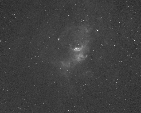
Frame 57: PSFSW = 0.001298 | PSFSNR = 0.004962
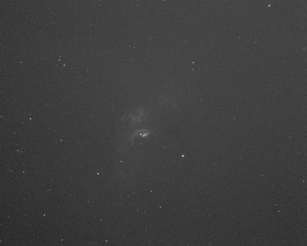
Frame 51: PSFSW = 6.796×10⁻⁵ | PSFSNR = 1.025×10⁻⁴
Frame 33: PSFSW = 0.002209 | PSFSNR = 0.004399
Frame 57: PSFSW = 0.001298 | PSFSNR = 0.004962
Figure 17 — Zoomed views of frames 33 (maximum PSFSW) and 57 (maximum PSF SNR). The higher mean FWHM in frame 57 has clearly penalized it for the PSFSW quality estimator. However, the PSF SNR estimator ignores signal concentration and hence is unaffected by star sizes, giving its maximum for frame 57 in this example. Contrarily to what may seem from this comparison, eccentricity (star elongation) is not an important factor here, since our implementation is able to measure total star fluxes by fitting elliptical PSF parameters to the shape and dimensions of each star.
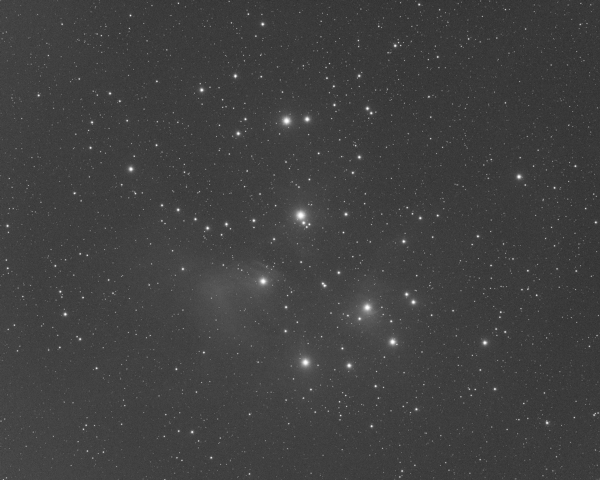
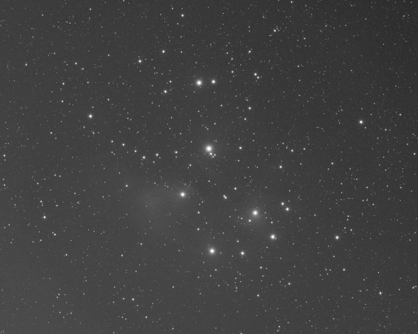
4.2 M45 / Red Channel
A set of 121 frames of M45 acquired with a Moravian G3-16200 CCD camera through a red filter by Edoardo Luca Radice. This set is interesting for quality estimation tests because it includes a small subset of images acquired under quite poor transparency conditions.
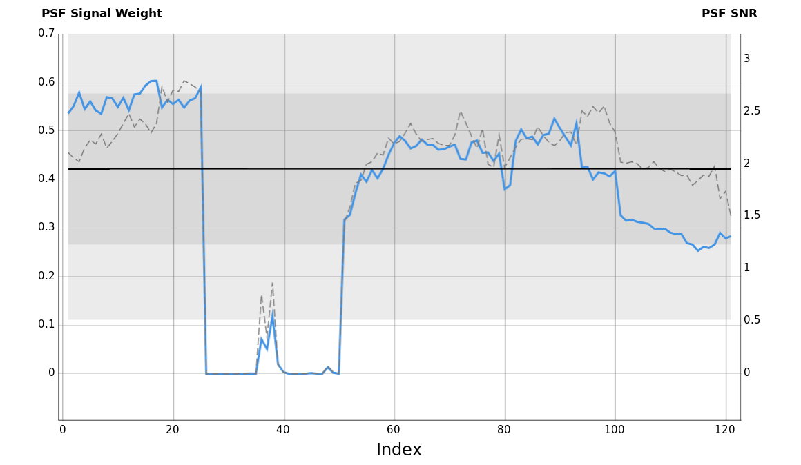
Figure 19 — M45 / Red data set: Selection of subframes
Frame 17: PSFSW = 0.605 | PSFSNR = 2.391

Frame 1: PSFSW = 0.537 | PSFSNR = 2.113
Frame 115: PSFSW = 0.254 | PSFSNR = 1.847
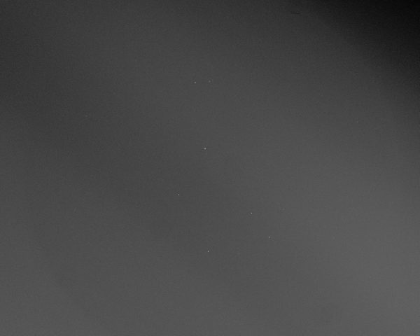
Frame 29: PSFSW = 2.405×10⁻⁷ | PSFSNR = 2.199×10⁻⁷
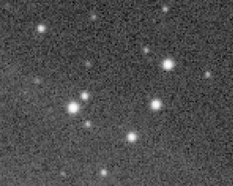
Figure 20 — Zoomed views of frames 17 (maximum PSFSW) and 115. The visible difference in image resolution between these two frames causes a substantial difference in PSFSW estimates (605 and 0.254, respectively), although not so much in PSF SNR estimates (2.391 and 1.847, respectively).
It is evident that the SNR estimator is not working correctly as a quality estimator for this data set. This is because the strong gradients in the subset of bad frames (frames 26–50) are being interpreted as signal by the SNR equation (see Equation [20]). The problem is not that SNR is wrong, but that SNR is not the appropriate estimator for this data set. In general, SNR cannot be used for image weighting for sets with differing strong gradients, as is the case in this example.
4.3 M81-M82 / Green Channel
A small set of 16 wide field frames of the M81/M82 region, acquired with a Finger Lakes ProLine PL16801 CCD camera through a green filter. The set was acquired under excellent sky conditions at the Astronomical Observatory of Aras de los Olmos (OAO), University of Valencia, Spain. Altitude above the horizon is in this case the main factor determining image quality.

Figure 22 — M81-M82 / Green data set: Selection of subframes
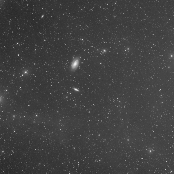
Frame 1: PSFSW = 3.741 | PSFSNR = 9.037
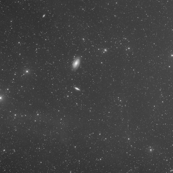
Frame 6: PSFSW = 3.070 | PSFSNR = 6.594

Frame 11: PSFSW = 2.458 | PSFSNR = 4.362
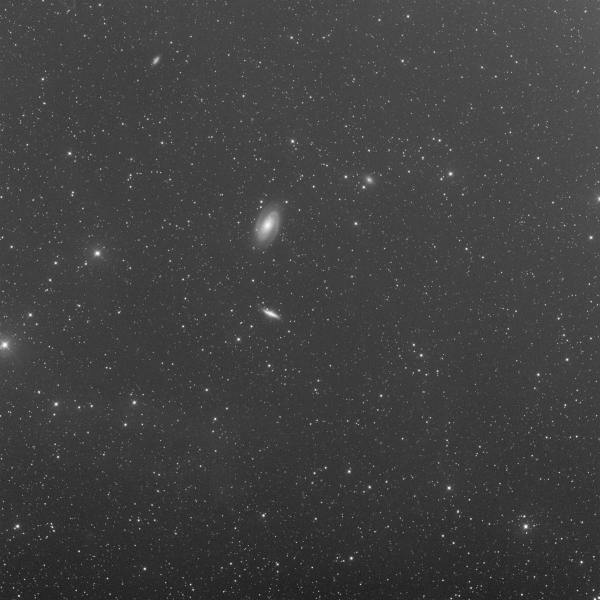
Frame 16: PSFSW = 2.130 | PSFSNR = 3.865
As expected, without other factors besides the natural variation in sky transparence due to the decreasing altitude, the PSF SNR and SNR estimators show high similarity.
4.4 M8 / OIII
A large set of 158 wide field frames of the M8 region, acquired with a STC Astro Duo-Narrowband filter and a ZWO ASI2600MC Pro OSC camera by Bernd Landmann. The data used for this example corresponds to the green channel of the demosaiced images, which captures most of the OIII line emission. These images have been acquired under excellent conditions from La Palma, Canary Islands, Spain.

Figure 24 — M8 / OIII data set: Selection of subframes
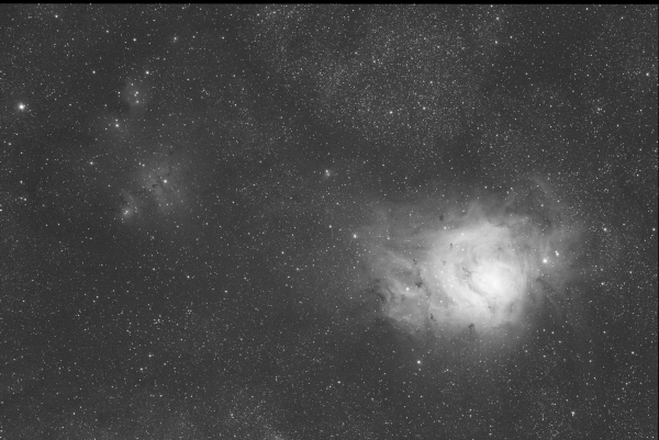
Frame 66: PSFSW = 1.8367 | PSFSNR = 1.3783
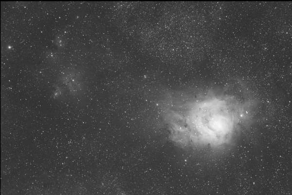
Frame 144: PSFSW = 0.9845 | PSFSNR = 1.4237
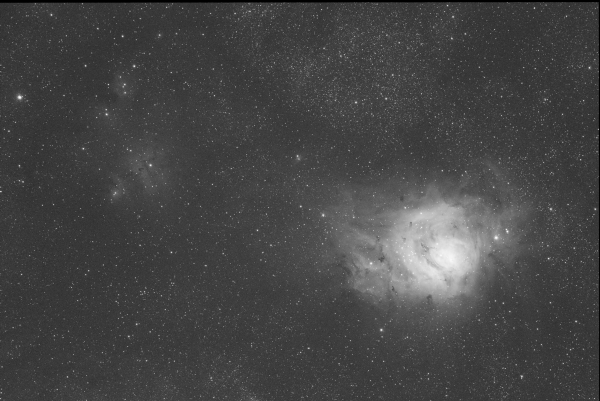
Frame 19: PSFSW = 1.2393 | PSFSNR = 0.7481
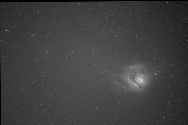
Frame 121: PSFSW = 0.0275 | PSFSNR = 0.0262

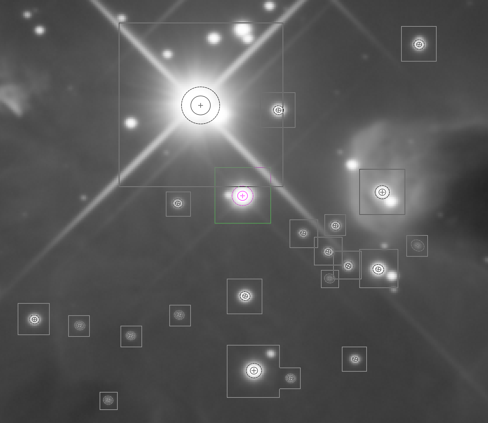
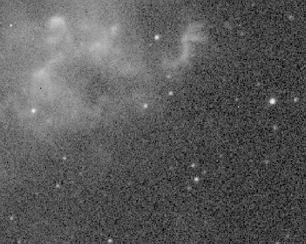
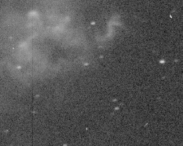
4.5 SH2-280 / H-α
In this example, we would discuss how the new image weighting algorithms balance image quality factors differently. The dataset consists of 74 light frames, with exposures of 600s and an H-α filter on the SH2–280 emission nebula. The dataset was taken in two separate nights where sky conditions visibly changed, and the passage of some clouds ruined the quality of a few frames. As usually happens under urban skies, image brightness due to light pollution changed significantly across the two nights. By plotting the image Median vs Altitude, we highlight how the overall image brightness evolved during the two sessions:
Figure 26 — SH2-280 / H-α data set: SubframeSelection Median vs Altitude graph

Image median value indicates the overall sky brightness. The first night was affected by the arrival of clouds that perturbed some frames in the middle of the session and completely ruined the last images (26–27–28). The sky was almost transparent on the second night, but light pollution appeared slightly higher than the first one.
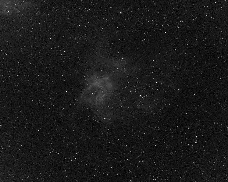


The light frames are spotted by black circles above with the same auto-stretch applied. On the left, the darkest image of the first session; in the middle one of the frames contaminated by the arrival of clouds; on the right, the darkest image of the second session.
Sky brightness acts as an additive light source that comes with its unavoidable shot noise: the higher the brightness, the higher the noise. This correlation is visible by depicting Noise vs Median:
Figure 27 — SH2-280 / H-α data set: SubframeSelection Median vs Noise graph
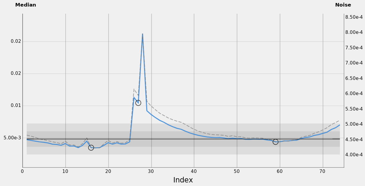
Image noise correlates to the median value as expected when the variation of the mean value is due to the presence of an additive light source, as sky brightness.
The impact of that additive brightness in terms of noise can be easily spotted by blinking the normalized images.
Figure 28 — A comparison between the registered/normalized two best frames of each night and a third frame strongly contaminated by the presence of clouds. The frames have been normalized with the LocalNormalization tool to make the visual noise comparison meaningful. While the noise of the best frames is visually similar, the contaminated frames are heavily dominated by sky shot noise.

PSF Flux and PSF Total Mean Flux measure the amount of star signal captured and how much that signal is concentrated. Showing the plot of these two properties and other quality measures highlights how powerful both are in capturing different aspects of image quality.
Figure 29 — A comparison of the stars between the registered best frames of the sessions and a frame strongly contaminated by clouds.
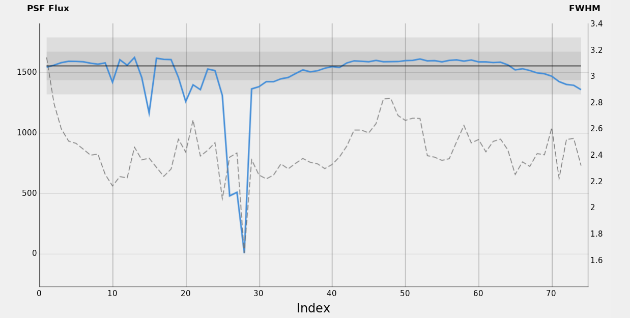
We identify a few significant phases within the whole session, where some PSF Flux properties can be highlighted.
Figure 30 — SH2-280 / H-α data set: Phase 1, clear sky with improving seeing.
Sky brightness regularly lowers as altitude increases. Almost no clouds contaminate the sky, thus FWHM is a good indicator of seeing and scope thermal adaptation. During the initial 60 minutes, FWHM lowers and the faintest stars become less blurry, increasing the number of detected stars accordingly. PSF Flux remains stable, indicating that sky transparency has not changed significantly.
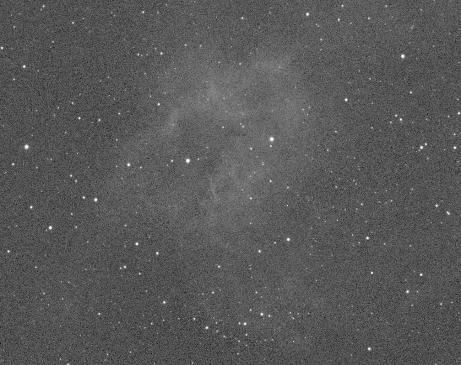
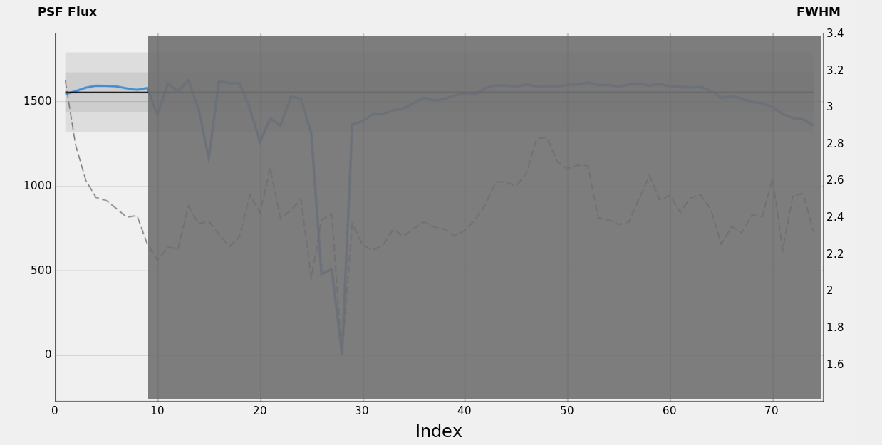
Figure 31 — SH2-280 / H-α data set: Phase 2, clouds arrival.
Clouds partially scatter and reflect the star's signal, reducing the overall flux received by the imaging sensor. In this second phase, some clouds have passed, and this is confirmed by inspecting the correlation between three factors: PSF Flux, number of detected stars, and sky median value. The strong correlation between these three factors hints that the source of the brightness increase should also be responsible for the star flux reduction and the reduction in the number of stars detected, all aspects following the presence of clouds.
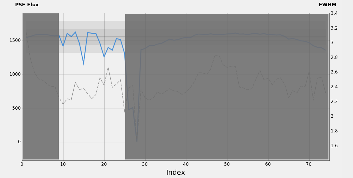
Figure 32 — SH2-280 / H-α data set: Phase 3, clouds ruined the images.
In this phase, the last frames of the first night have been strongly deteriorated by the presence of clouds. Images are dominated by the scatter noise and all image quality indicators like FWHM, number of stars, PSF Flux, and median coherently tend towards the worst values. In this situation, the weak correlation between FWHM and PSF Flux suddenly becomes strong.
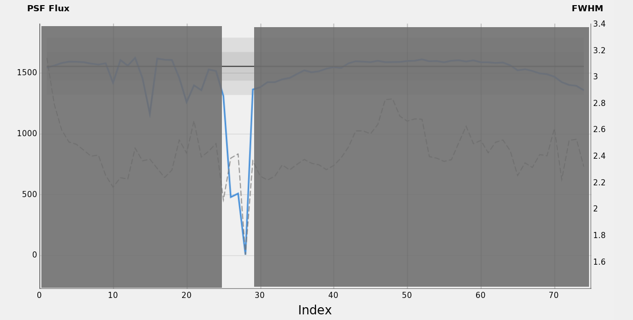
Figure 33 — SH2-280 / H-α data set: Phase 4, a night with a clear sky.
This phase corresponds to the entire second night of the shooting. This phase is characterized by the absence of clouds, which provides the ideal condition to inspect how the PSF Flux measure works under a clear sky. As expected, star flux depends on sky transparency, with a weak dependency on small seeing fluctuations. This is confirmed by the graphs, which show a very regular and smooth behaviour of PSF Flux values that are mainly correlated to the part of the sky pointed during the session and to the correspondent atmospheric properties. Given the ideal conditions, we assume FWHM is a good indicator of seeing: we can see that the seeing has a stable trend around 2.4 px, with some fluctuations that are quite uncorrelated to PSF Flux.
The above analysis on PSF Flux can be summarized with the following statements:
- The PSF Flux property shows a strong correlation with sky transparency (atmospheric absorption and presence of clouds) and a weak correlation with seeing (FWHM)
- The presence of strong clouds affecting the images turns the weak correlation between PSF Flux and FWHM into a strong correlation.
PSF Total Mean Flux measures how much star flux is concentrated into the inner part of the PSF, thus being related to image definition: the higher its value, the sharper the stars. By plotting PSF Total Mean Flux vs FWHM the strong correlation between both properties becomes evident:
Figure 34 — SH2-280 / H-α data set: PSF Total Mean Flux vs FWHM.

The strong inverse correlation between PSF Total Mean Flux and FWHM is obvious.
Although this is generally true, when FWHM is reduced because of the presence of clouds which reduce the overall star flux, that inverse correlation becomes a positive one, and the two measures show the same trends, as happens in frame 28.
We have now all the ingredients to properly discuss how the different weighting algorithms work with the images of this data set:
Figure 35 — SH2-280 / H-α data set: PSF Signal Weight vs PSF SNR.
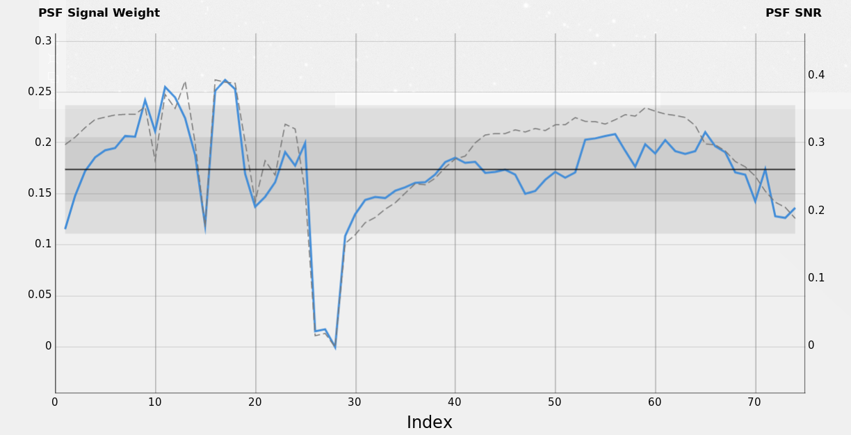
PSF Signal Weight and PSF SNR show an overall good correlation; in particular, both penalize images where star flux is strongly reduced because of the presence of the clouds. The latter is a very new behaviour that is not taken into account by a standard SNR weighting algorithm. The two methods differ by the PSF Total Mean Flux's role in the PSF Signal Weight formula.
PSF Signal Weight penalizes more frames from 1 to 8 because they have a higher FWHM, while PSF SNR takes into account only the overall total star flux. PSF Signal Weight also fluctuates accordingly with the inverse trend of FWHM in the second night, while PSF SNR closely follows the trend of the overall star flux.
The comparison between PSF Signal Weight and PSF SNR shows the advantages provided by both methods, along with the differences:
- Both PSF Signal Weight and SNR penalize images affected by clouds, where the star flux is strongly reduced.
- PSF SNR relies on the overall star flux and is less sensitive to how much the signal is concentrated.
- PSF Signal Weight takes into account signal concentration (i.e. definition) and promotes image with higher resolution.
Depending on the objective, one weighting method could be preferable against the other.
Finally, SNR represents the legacy SNR weighting method based on the overall signal-to-noise ratio. The method can be adopted with images that are not contaminated by clouds since the overall signal measurement cannot distinguish between the target and the sky signal, resulting in higher weights assigned to degraded images, as depicted in the following comparison graph:
Figure 36 — SH2-280 / H-α data set: PSF Signal Weight vs SNR.

SNR is based on the measurement of the image's overall signal. Being positively affected by gradients and sky brightness, the result keeps promoting brighter images where the actual target signal-to-noise ratio is low. Moreover, SNR cannot reject very bright images where the target signal is entirely buried under the noise.
The PSF Signal Weight algorithm is capable of synthesizing different quality factors into a single variable, balancing both signal-to-noise ratio and image definition. PSF SNR is a robust alternative to the standard SNR weighting algorithm.
Both methods are capable of capturing and penalizing images that have been deteriorated by the presence of clouds, overcoming the limitations of a purely SNR-based weighting method.
5 Linear Regression Analysis
[hide]
Contributed by John Pane
This analysis explores the value added by PSF Signal Weight (PSFSW) by evaluating its relationship to other variables that have historically been used to evaluate image quality. The strategy is to use linear regression to discover whether, and how well, PSFSW can be replicated using those previously-available variables.
The particular eight variables examined are: Stars, FWHM, Eccentricity, Median, Altitude, SNR, Noise, and Median Mean Deviation (SNR was previously called SNR Weight). For each of these, the relationship to PSFSW might be linear or non-linear, and direct or inverse—for example: Stars, Stars2, 1/Stars and 1/Stars2. Including these variants of the original eight variables expands the set to 32 variables.
These 32 variables offer 232 possible combinations that might come close to replicating PSFSW. This set could be expanded further, to include the products of two variables (e.g., Stars/FWHM), higher-order polynomials, or other transformations such as logarithms. We will find that to be unnecessary for obtaining a good approximation of PSFSW.
The analysis proceeds by using a variable selection algorithm to search for a minimal set of the 32 variables that can closely replicate PSFSW. This proceeds in two steps, first to iteratively add and remove variables to minimize a statistical metric called Akaike information criteria (AIC).[9] AIC strikes a balance between fitting the data well and using fewer variables. The second step accepts slightly poorer model fit to enable further reduction in the number of variables used. This is done by iteratively removing variables with relatively weaker relationships to PSFSW based on p-values,[10] until all the remaining variables have p < 0.0001. This is a very conservative criterion—in common practice p-values as high as 0.05 are considered to be statistically significant.
Running this algorithm across six different datasets produces six unique regression equations that very closely replicated PSFSW, using as few as three variables and as many as eleven. In most cases, the regression has an adjusted R2[11] greater than 99%, meaning the equation explains more than 99% of the variance in PSFSW. Values of R2 this high indicate an excellent statistical fit.
Among the datasets explored, the lowest R2 was 95%, still a very good fit. For this dataset, step 1 identified seven variables and step 2 trimmed the list to three. The regression results imply that if a user entered the following weight expressions in SubframeSelector, they would come very close to replicating PSFSW:
 [22]
[22]This is demonstrated by plotting PSFSW versus the equation’s approximation, as shown in Figure [37].
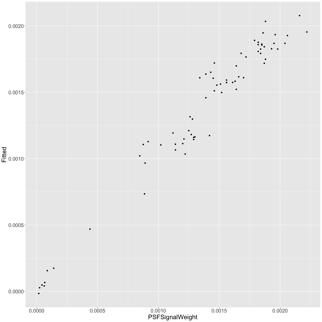
Figure 37 — A plot of PSF Signal Weight versus the approximation given by Equation [22]. If the model were perfect, the points would be on the 45-degree diagonal.
Because the variables are on different scales, it may be challenging to understand the relative importance, or weight, of the various terms. To reveal this information all the variables can be standardized without compromising the regression—specifically, they can be rescaled to have a mean of zero and standard deviation of one. The regression coefficients then represent relative weights, as seen in Table 2.
SNR2 and SNR individually receive about eight times as much weight as Stars, though they have opposite signs so their combined weight is not as large as their individual weights. Another use for these standardized coefficients is to interpret how much PSFSW is influenced by changes in one of the independent variables. As an example, a one-standard-deviation increase in Stars results in a half-standard-deviation increase in the estimated PSFSW.
For six datasets explored using this technique, the following table shows the resulting equations, and the percentage of PSFSW variance explained:
|
Equation |
Variance explained |
|---|---|
 |
99.5% |
 |
99.7% |
 |
99.1% |
 |
95.4% |
 |
99.8% |
 |
99.3% |
It can be seen that, although the variables previously available in SubframeSelector are able to very accurately approximate PSF Signal Weight, the equations vary drastically from dataset to dataset—presumably due to variations in the conditions and equipment. A similar analysis predicting PSFSNR produces similar results: drastically different equations with four to nine variables that explain 90.6% to 99.8% of the variance in PSFSNR.
The next exploration is to merge these six datasets (with a total of 711 subframes) and run the same analysis. A more complex equation with 19 variables is produced, which explains about 90% of the variance in PSFSW in the combined dataset. If this equation is then used to predict PSFSW in each individual dataset, the following percentages of variance are explained: 99.4, 98.2, 99.7, 98.8, 96.2, and 99.8.
This suggests that perhaps a general equation could be found that would work well in approximating PSFSW (or PSFSNR) in all datasets. More data would be needed to find that equation, and it would likely be even more complex than 19 variables. (It should be noted, though, that an equation with N variables will only work on datasets with more than N subframes. So there is good reason not to allow the number of variables to get too large.) The true test of such a “universal” equation would be if it work wells for new datasets that were not part of the large dataset used to generate the equation. Thankfully, we do not need to find a “universal” equation to approximate PSFSW because the exact quantity is now available directly in PixInsight.
This analysis does not prove that PSFSW is the best metric for evaluating image quality. However, if other analyses show it to be excellent for that purpose, it should be considered a major advance because it seems to automatically capture the important dimensions of image quality in a single metric.
This analysis was performed using ordinary least squares regression in the free R statistical software package,[12] with the olsrr extension[13] to implement the automatic variable selection process. Of course, linear regression can be performed in any statistical software package and even such software as Microsoft Excel.[14]
Note: Some readers may be concerned that variables in these regression models are collinear. This would be a concern if we were attaching great importance to the coefficient estimates or the statistical significance of particular variables. However, our focus in this analysis is the predictive power or reliability of the model as a whole, for which collinearity or multicollinearity[15] are not a concern.
References
[1] Wikipedia article: Levenberg–Marquardt algorithm
[2] Moffat, A. F. J. (1969). A Theoretical Investigation of Focal Stellar Images in the Photographic Emulsion and Application to Photographic Photometry. Astronomy and Astrophysics, Vol. 3, p. 455
[3] Starck, J.-L., Murtagh, F. and J. Fadili, A. (2010). Sparse Image and Signal Processing: Wavelets, Curvelets, Morphological Diversity. Cambridge University Press. https://doi.org/10.1017/CBO9780511730344
[4] Jean‐Luc Starck and Fionn Murtagh (1998). Automatic Noise Estimation from the Multiresolution Support. Publications of the Royal Astronomical Society of the Pacific, vol. 110, pp. 193–199
[5] Rousseeuw, P. J., & Croux, C. (1993). Alternatives to the Median Absolute Deviation. Journal of the American Statistical Association, 88(424), 1273–1283. https://doi.org/10.2307/2291267
[6] Rand R. Wilcox (2021). Introduction to Robust Estimation and Hypothesis Testing, Fifth Edition. Section 3.1. Copyright © 2022 Elsevier Inc. All rights reserved. https://doi.org/10.1016/C2019-0-01225-3
[7] Maples, M. et al. (2018). Robust Chauvenet Outlier Rejection. The Astrophysical Journal Supplement Series. 238. 2. https://doi.org/10.3847/1538-4365/aad23d
[8] Wikipedia article: Inverse-variance weighting
[9] Wikipedia article: Akaike information criterion
[10] Wikipedia article: p-value
[11] Wikipedia article: Adjusted R2
[12] Website: The R Project for Statistical Computing
[13] Website: olsrr: Tools for Building OLS Regression Models
[14] Website: Excel regression tutorial
[15] Wikipedia article: Multicollinearity
Copyright © 2022 Pleiades Astrophoto. All Rights Reserved.