PixelMath is one of those tools that really define PixInsight as a uniquely powerful image processing platform. My intention with this tool has always been to realize the idea of flexibility with your imagination being the only limit, and this new version makes that idea come true as never before. In this post I'm going to show you some important new features implemented in version 1.8.0 of PixelMath, which is now available as a regular update to version 1.8.8-7 of PixInsight on all supported platforms.
Generators
Generators are special functions that can build new images on the fly when a PixelMath expression is executed. This is a completely new feature that radically changes the applicability and meaning of PixelMath, which is from now on much more than a pixel-by-pixel image manipulation tool. With this feature, PixelMath evolves to become an extremely powerful image processing and analysis tool.
To understand how generators work, let's see first how images play their role in PixelMath expressions. As you know, images have always been native objects of the PixelMath language. For example, the following expression:
0.75*this + 0.25*other
combines the 'this' and 'other' images in a ratio of 3/4 to 1/4. Images are specified by their identifiers in PixelMath expressions. I'm sure all of you have seen expressions like this one many times, since this is standard practice to implement narrowband combinations.
So we can use existing images very easily, by just putting their names in a PixelMath expression. However, suppose that we want to use a transformed version of an existing image, instead of the image itself. Or a transformed version of a transformed version, and so on. For example, a high-pass filter can be implemented by subtracting a low-pass filtered version of an original image. An example is shown in the following figure:
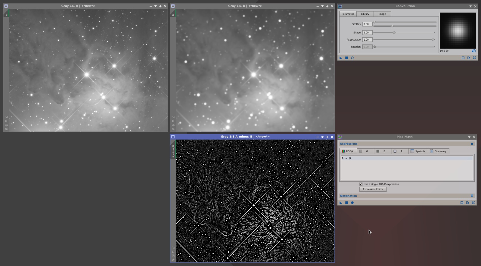
Here we have an image 'A' and its duplicate 'B', to which we have applied a convolution with a Gaussian filter (which is a low-pass filter, as you know). The image 'A_minus_B' is the result of subtracting B from A with PixelMath. The 'A_minus_B' image is now a high-pass filtered version of 'A', since we have removed low-pass components. This is similar to how a classical unsharp mask filter works.
Now, wouldn't it be nice to have this functionality implemented directly in PixelMath, that is, without needing to duplicate images, apply other processes, and repeat the same sequence each time we want to try out different parameters, such as the Gaussian filter size in this particular example? Yes, it is extremely nice, and it is now a reality. See it in action on the following figure:
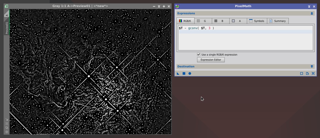
The PixelMath expression used in the above example is:
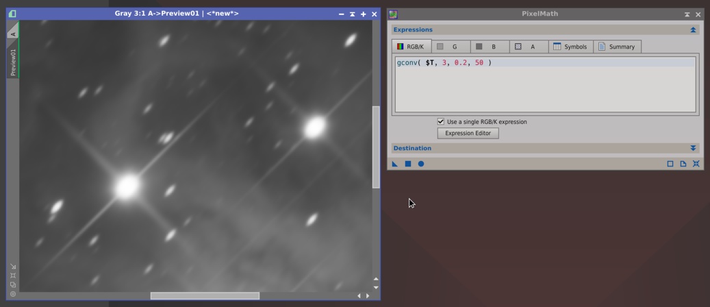
gconv() is one of the new PixelMath generators. It performs a convolution of the specified image with a Gaussian filter and generates a new image with the convolution result. The newly generated image plays exactly the role of an existing image in the PixelMath expression to which the generator belongs. This example is simple, since gconv() is capable of much more sophistication, such as applying elliptical filters with prescribed aspect ratios and rotation angles:
I'll describe gconv() and the rest of generators later in this post. You have all of them well documented in the Expression Editor dialog.
Generators are always executed just after all image references, metasymbols and invariant subexpressions have been evaluated, but before running PixelMath expressions. This means that generators don't have the concept of current pixel, as the rest of PixelMath functions and operators do: a generator works on an entire image as a single step just once, not in a pixel-by-pixel fashion as normal functions. This has important consequences that must be taken into account from the syntactic and semantic points of view. One of them is that variables cannot be used to define generator parameters. However, constants can be used without problems. For example, the following is valid:
But the following is illegal:
because now rotationAngle has been defined (and is being used) as a variable. If the above expression were legal, we would have a set of potentially infinite generated images during expression execution, which obviously does not make any sense. For the same reason, an image identifier (including metasymbols such as $T) can only be used to define the source image of a generator, but not any of its other working parameters (because no generator can work on two or more images in the same function call, for now). For example:
is an illegal attempt to use the image 'MyMatrixOfSigmaValues' to define the standard deviation of the Gaussian filter. Good try, we would say
Another limitation is that you cannot use a channel selector with a generator. The following is not valid:
The reason is that the PixelMath lexical analyzer treats gconv() as a function call and is unable to identify it as an image reference, hence the use of a channel selector is detected as a syntax error. A future version may overcome this limitation.
You can, however, select a single channel of an existing image as the source of a generator. The following is syntactically valid, and would work if $T has two or more channels:
The above expression would convolve the second channel of $T to generate a new grayscale, single-channel image with the result.
Now that we know what generators are and how they can be used in PixelMath expressions, let's enumerate the generators available in this version, with a few examples.
Available Generators
Convolution of the specified image with a box average filter of odd size n ≥ 3.
The specified image with its pixel sample values binarized with respect to the threshold value t. For each pixel sample v, the corresponding binarized sample value v' is given by:
v' = 0 if v < t
v' = 1 if v ≥ t
Dilation morphological filter with odd filter size n ≥ 3 and structuring element str, applied to the specified image.
Erosion morphological filter with odd filter size n ≥ 3 and structuring element str, applied to the specified image.
Convolution of the specified image with an elliptical Gaussian filter:
Horizontal mirror (or horizontal reflection) of the specified image.
Convolution of the specified image with a custom kernel filter.
The arguments k_ij are filter kernel elements specified in row-major order. The minimum kernel size is 3×3, hence at least 9 elements must be defined. For the smallest 3×3 kernel we have the following filter configuration:
k11 k12 k13
k21 k22 k23
k31 k32 k33
Filter kernels must be square matrices with odd dimensions, so valid kernel sizes are 3×3, 5×5, 7×7, etc.
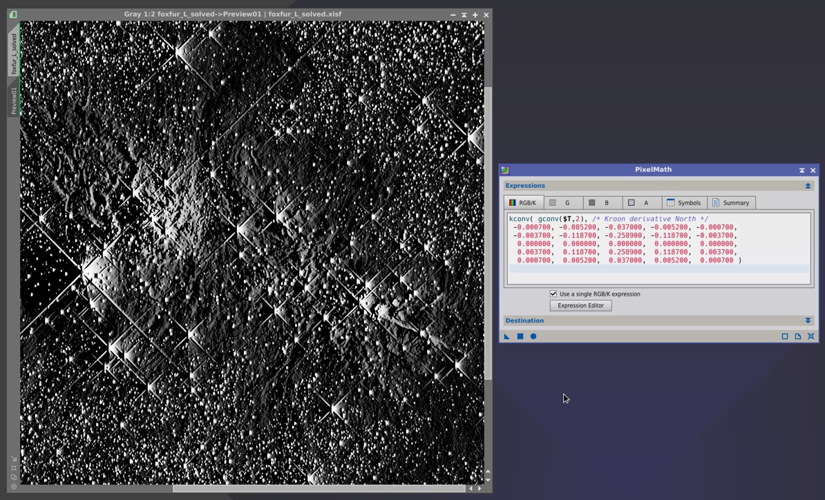
For example, the following PixelMath expression applies two successive convolutions: a first one with a Gaussian filter, and a second one with a high-pass filter kernel:
Local variance map of the specified image with odd window size d ≥ 3 pixels and kernel function k.
A local variance map is a sensitive analysis tool to explore the distribution of pixel intensity variations at small scales. This allows for the implementation of subtle adaptive procedures with PixelMath. For example, the following expression:
applies a median filter selectively to pixels where the local variance is below a prescribed threshold t, which depends on the target image and must be found experimentally. For example, t=1e-8 can be a good starting value for a linear deep-sky image. The expression above implements a powerful noise reduction procedure. More sophisticated, adaptive noise filtering processes based on the same technique can be designed with iswitch() constructs. The following figure shows a good example (please click on the image to see a full-size version).
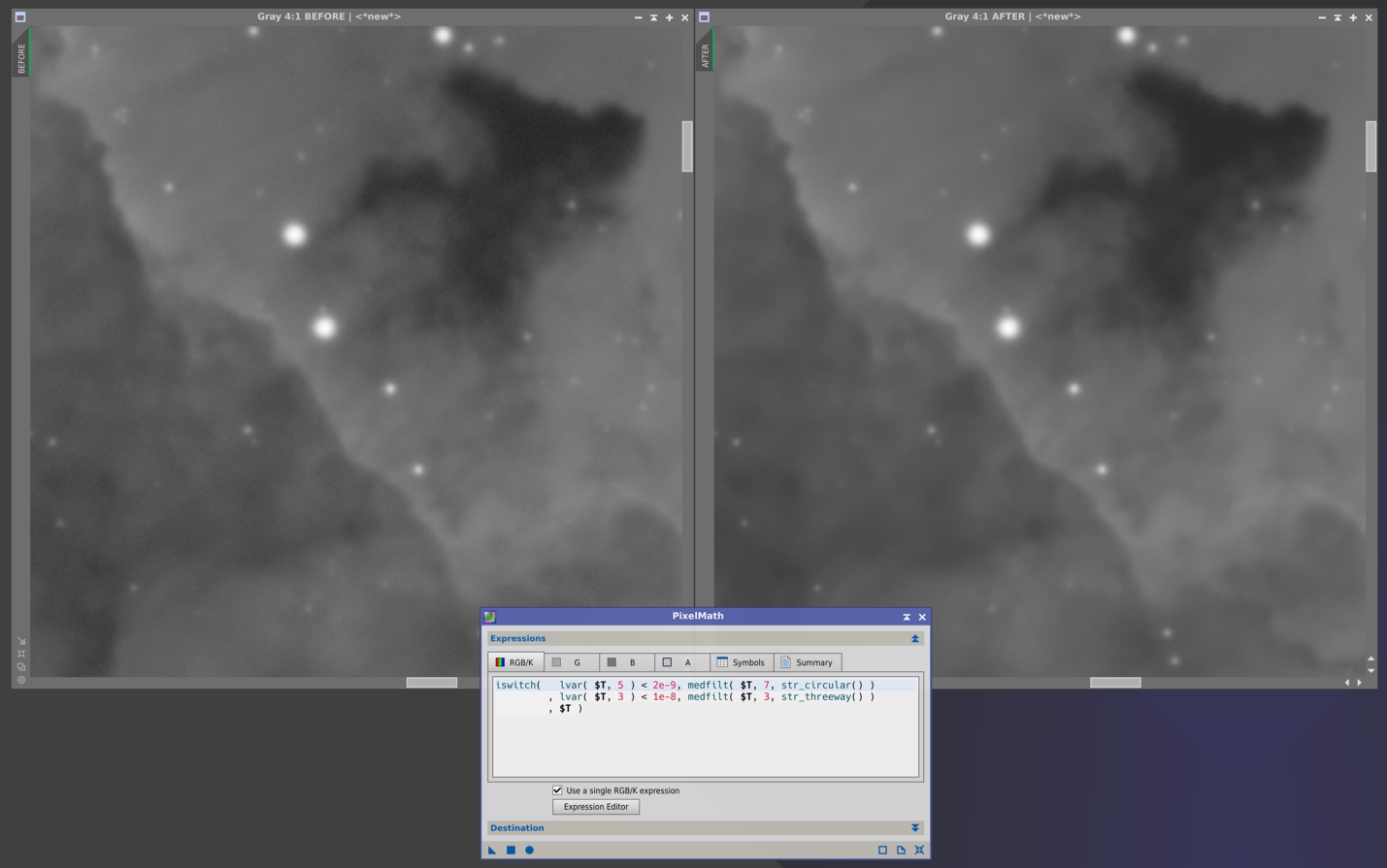
The expression used in this example is:
Local variance maps are always generated as 64-bit floating point images. This ensures that no truncation or round-off errors will degrade their ability to represent subtle intensity variations, which is especially important for linear images.
Morphological median filter with odd filter size n ≥ 3 and structuring element str, applied to the specified image.
The specified image with its pixel sample values scaled linearly to the range [a,b]. For each pixel sample v, the corresponding normalized value v' is given by:
v' = a + (b - a)×(v - m)/(M - m)
where m and M are, respectively, the minimum and maximum pixel sample values in the image before normalization.
Rotation of an image by the specified angle in degrees, with center of rotation located at (dx,dy) coordinates measured in pixels from the geometric center of the image. If no center coordinates are specified, the default center of rotation is (0,0), which corresponds to the geometric center of the image.
Translation of an image by the specified increments dx and dy, respectively in the horizontal (X-axis) and vertical (Y-axis) directions. In the next example I have implemented an interesting edge detector using multiple translations in an 8-connected neighborhood. Again, please click the image to see a full-size version.
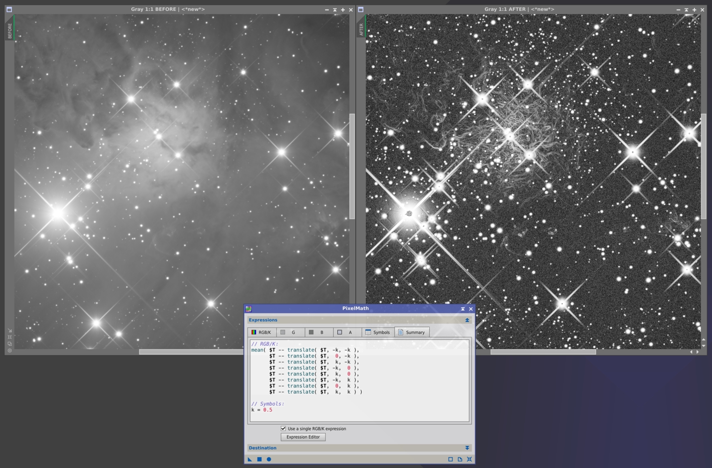
In case you want to play with this idea, here is the expression:
where the symbol k is the translation distance in pixels (k=0.5 in the example above).
The specified image with its pixel sample values truncated to the range [a,b]. For each pixel sample v, the corresponding truncated sample value v' is given by:
v' = a if v < a
v' = b if v > b
v' = v if a ≤ v ≤ b
Vertical mirror (or vertical reflection) of the specified image.
Image Cache
The new version of PixelMath comes with another important new feature: a cache of generated images. When the image cache is enabled, generated images are preserved before and after PixelMath execution. This option is useful to speed up calculations when PixelMath expressions using generators are being executed repeatedly (for example, on a preview to fine tune expressions by trial/error work). Note that this uses memory resources, which may become quite significant, especially after many executions of PixelMath expressions with varying generator function parameters.
The image cache is disabled by default. When it is disabled, existing generated images will be destroyed before and after PixelMath execution, so they'll have to be recalculated in successive executions of the same expressions.
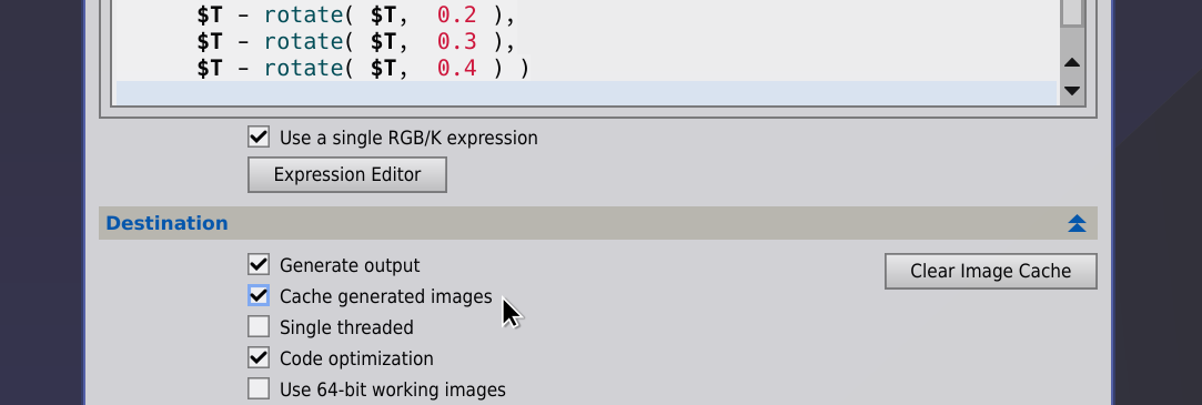
The new Cache generated images check box and the Clear Image Cache button allow you to manage the image cache as required.
Structure and Kernel Selection Functions
The following functions can be used with the medfilt(), erosion() and dilation() generators to select a structuring element to apply the corresponding morphological operators:
The following functions can be used with the lvar() generator to select a kernel function for local variance calculation:
The documentation for all of these functions included in the Expression Editor dialog provides detailed information with examples.
Improved Statistics Calculation Functions
All statistics calculation functions, such as med(), mdev(), mean(), min(), max(), etc, include now an optional set of 4 parameters to define a rectangular region of interest. For example, this is now the definition of the med() function when applied to calculate the median pixel value of an image:
the optional x0, y0, w, and h parameters define a rectangular region of interest (ROI). These parameters are, respectively, the left coordinate, the top coordinate, the width and the height of the ROI, all of them expressed in integer pixel units. If a ROI is specified, the median pixel sample value will be computed exclusively for pixel samples within the intersection between the ROI and the image bounds. If no ROI is specified, the median pixel sample value will be computed for the entire image.
Here is a complete list with all image statistics calculation functions:
Average absolute deviation from the median.
Mean of squares.
Biweight midvariance (BWMV).
Maximum pixel sample value.
Median absolute deviation from the median (MAD).
Arithmetic mean of pixel sample values.
Median of pixel sample values.
Minimum pixel sample value.
Norm, or the sum of pixel sample values.
Percentage bend midvariance.
Qn scale estimator of Rousseeuw and Croux.
Standard deviation from the mean.
Sn scale estimator of Rousseeuw and Croux.
Sum of square pixel sample values.
Variance from the mean.
New Symbol Definition Functions
Version 1.8.0 adds two useful symbol definition functions that allow you to use environment variables directly in PixelMath expressions:
The symbol will be initialized with the value of the specified environment variable var converted to a scalar. For example, suppose you have executed the following command on Linux, macOS, or on any operating system from PixInsight's Process Console window:
or on Windows:
Then you can include the following to define a constant 'thr' in PixelMath:
and of course you can use thr in your PixelMath expression. Each occurence of thr will be replaced with the constant 0.273 automatically before expression execution.
The value of symbol will be either one, if the specified environment variable is currently defined for the running process with a non-empty value, or zero otherwise.
New Line Comments
C++ line comments (with the '//' prefix) are now supported in PixelMath expressions, along with the previously supported C-style block comments (with the '/*' and '*/' delimiters). For example, this is now a valid expression:
Improved Expression Editor Dialog
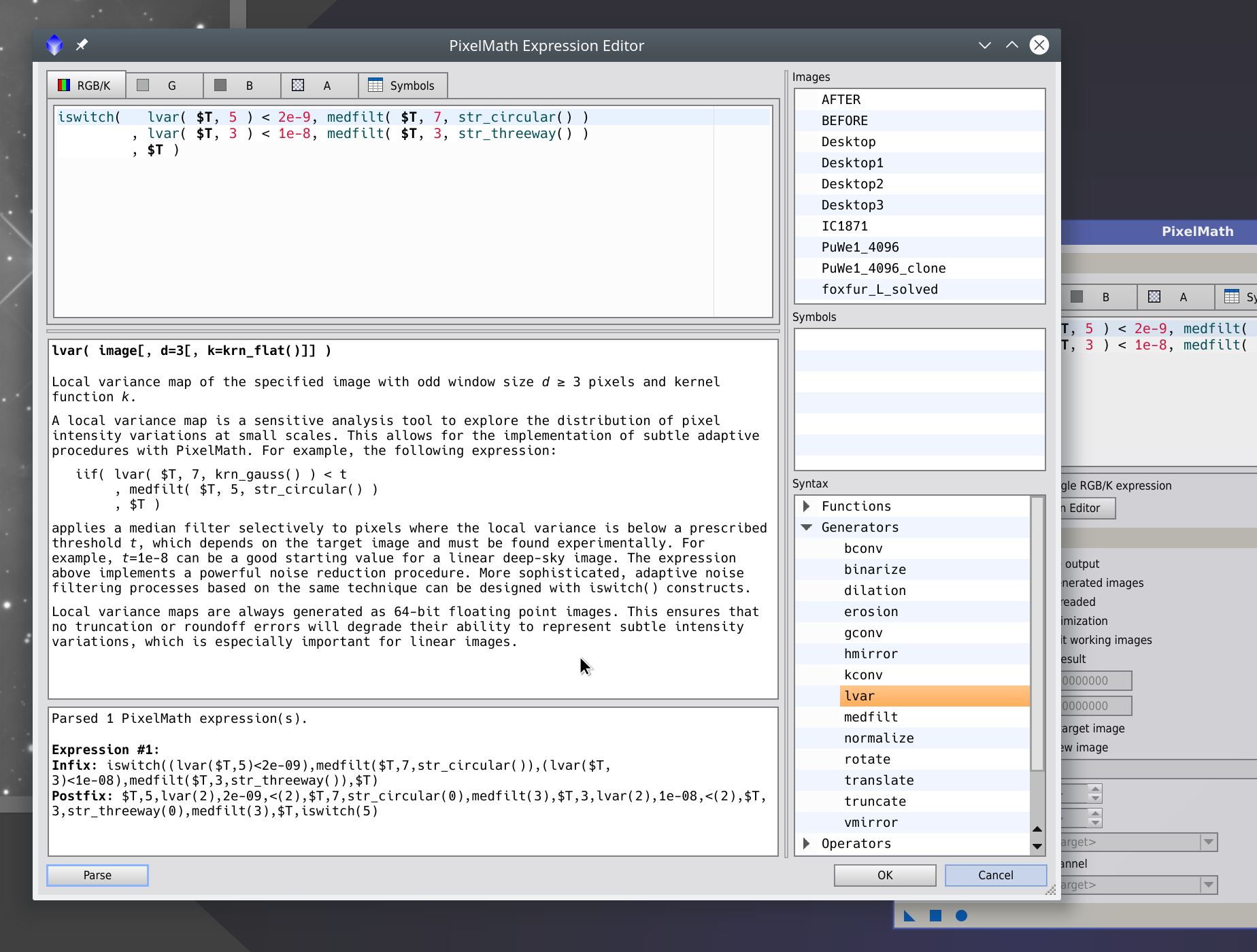
The Expression Editor dialog has now two splitters that allow you to resize the documentation panel and the right panel, where images, symbols and syntax elements can be selected.
The Syntax tree includes now all functions, generators, operators, punctuators, symbol definition functions and metasymbols that form part of the PixelMath language. The documentation for all functions, generators and operators has been considerably improved with more detailed descriptions and examples.
____________________
I hope you'll find all of this work useful and stimulating for your creativity. Thank you for your attention.
Generators
Generators are special functions that can build new images on the fly when a PixelMath expression is executed. This is a completely new feature that radically changes the applicability and meaning of PixelMath, which is from now on much more than a pixel-by-pixel image manipulation tool. With this feature, PixelMath evolves to become an extremely powerful image processing and analysis tool.
To understand how generators work, let's see first how images play their role in PixelMath expressions. As you know, images have always been native objects of the PixelMath language. For example, the following expression:
0.75*this + 0.25*other
combines the 'this' and 'other' images in a ratio of 3/4 to 1/4. Images are specified by their identifiers in PixelMath expressions. I'm sure all of you have seen expressions like this one many times, since this is standard practice to implement narrowband combinations.
So we can use existing images very easily, by just putting their names in a PixelMath expression. However, suppose that we want to use a transformed version of an existing image, instead of the image itself. Or a transformed version of a transformed version, and so on. For example, a high-pass filter can be implemented by subtracting a low-pass filtered version of an original image. An example is shown in the following figure:

Here we have an image 'A' and its duplicate 'B', to which we have applied a convolution with a Gaussian filter (which is a low-pass filter, as you know). The image 'A_minus_B' is the result of subtracting B from A with PixelMath. The 'A_minus_B' image is now a high-pass filtered version of 'A', since we have removed low-pass components. This is similar to how a classical unsharp mask filter works.
Now, wouldn't it be nice to have this functionality implemented directly in PixelMath, that is, without needing to duplicate images, apply other processes, and repeat the same sequence each time we want to try out different parameters, such as the Gaussian filter size in this particular example? Yes, it is extremely nice, and it is now a reality. See it in action on the following figure:

The PixelMath expression used in the above example is:
$T - gconv( $T, 3 )gconv() is one of the new PixelMath generators. It performs a convolution of the specified image with a Gaussian filter and generates a new image with the convolution result. The newly generated image plays exactly the role of an existing image in the PixelMath expression to which the generator belongs. This example is simple, since gconv() is capable of much more sophistication, such as applying elliptical filters with prescribed aspect ratios and rotation angles:

I'll describe gconv() and the rest of generators later in this post. You have all of them well documented in the Expression Editor dialog.
Generators are always executed just after all image references, metasymbols and invariant subexpressions have been evaluated, but before running PixelMath expressions. This means that generators don't have the concept of current pixel, as the rest of PixelMath functions and operators do: a generator works on an entire image as a single step just once, not in a pixel-by-pixel fashion as normal functions. This has important consequences that must be taken into account from the syntactic and semantic points of view. One of them is that variables cannot be used to define generator parameters. However, constants can be used without problems. For example, the following is valid:
Code:
Symbols:
sigma = 2.5, aspectRatio = 0.2, rotationAngle = 43

Expression:
gconv( MyImage, sigma, aspectRatio, rotationAngle )
But the following is illegal:
Code:
Symbols:
sigma = 2.5, aspectRatio = 0.2, rotationAngle

Expression:
rotationAngle = 180*atan( y(), x() )/pi();
gconv( MyImage, sigma, aspectRatio, rotationAngle )
because now rotationAngle has been defined (and is being used) as a variable. If the above expression were legal, we would have a set of potentially infinite generated images during expression execution, which obviously does not make any sense. For the same reason, an image identifier (including metasymbols such as $T) can only be used to define the source image of a generator, but not any of its other working parameters (because no generator can work on two or more images in the same function call, for now). For example:
gconv( MyImage, MyMatrixOfSigmaValues, aspectRatio, rotationAngle )is an illegal attempt to use the image 'MyMatrixOfSigmaValues' to define the standard deviation of the Gaussian filter. Good try, we would say
Another limitation is that you cannot use a channel selector with a generator. The following is not valid:
gconv( $T )[1]The reason is that the PixelMath lexical analyzer treats gconv() as a function call and is unable to identify it as an image reference, hence the use of a channel selector is detected as a syntax error. A future version may overcome this limitation.
You can, however, select a single channel of an existing image as the source of a generator. The following is syntactically valid, and would work if $T has two or more channels:
gconv( $T[1] )The above expression would convolve the second channel of $T to generate a new grayscale, single-channel image with the result.
Now that we know what generators are and how they can be used in PixelMath expressions, let's enumerate the generators available in this version, with a few examples.
Available Generators
bconv( image[, n=3] )Convolution of the specified image with a box average filter of odd size n ≥ 3.
binarize( image[, t=0.5] )The specified image with its pixel sample values binarized with respect to the threshold value t. For each pixel sample v, the corresponding binarized sample value v' is given by:
v' = 0 if v < t
v' = 1 if v ≥ t
dilation( image[, n=3[, str=str_square()]] )maxfilt( image[, n=3[, str=str_square()]] )Dilation morphological filter with odd filter size n ≥ 3 and structuring element str, applied to the specified image.
erosion( image[, n=3[, str=str_square()]] )minfilt( image[, n=3[, str=str_square()]] )Erosion morphological filter with odd filter size n ≥ 3 and structuring element str, applied to the specified image.
gconv( image[, sigma=2[, rho=1[, theta=0[, eps=0.01]]]] )Convolution of the specified image with an elliptical Gaussian filter:
- sigma: Standard deviation of the filter distribution on its major axis (sigma > 0).
- rho: The ratio between the minor and major axes of the generated filter distribution (0 ≤ rho ≤ 1).
- theta: Rotation angle of the major filter axis in degrees (−180° ≤ theta ≤ 180°). Ignored when rho = 1.
- eps: Maximum truncation error of computed filter coefficients (eps > 0).
hmirror( image )Horizontal mirror (or horizontal reflection) of the specified image.
kconv( image, k11, k12, k13, k21, k22, k23, k31, k32, k33[, ...] )Convolution of the specified image with a custom kernel filter.
The arguments k_ij are filter kernel elements specified in row-major order. The minimum kernel size is 3×3, hence at least 9 elements must be defined. For the smallest 3×3 kernel we have the following filter configuration:
k11 k12 k13
k21 k22 k23
k31 k32 k33
Filter kernels must be square matrices with odd dimensions, so valid kernel sizes are 3×3, 5×5, 7×7, etc.
For example, the following PixelMath expression applies two successive convolutions: a first one with a Gaussian filter, and a second one with a high-pass filter kernel:
Code:
kconv( gconv($T,2), /* Kroon derivative North */
-0.000700, -0.005200, -0.037000, -0.005200, -0.000700,
-0.003700, -0.118700, -0.258900, -0.118700, -0.003700,
  0.000000,  0.000000,  0.000000,  0.000000,  0.000000,
  0.003700,  0.118700,  0.258900,  0.118700,  0.003700,
  0.000700,  0.005200,  0.037000,  0.005200,  0.000700 )
lvar( image[, d=3[, k=krn_flat()]] )Local variance map of the specified image with odd window size d ≥ 3 pixels and kernel function k.
A local variance map is a sensitive analysis tool to explore the distribution of pixel intensity variations at small scales. This allows for the implementation of subtle adaptive procedures with PixelMath. For example, the following expression:
Code:
  iif( lvar( $T, 7, krn_gauss() ) < t
        , medfilt( $T, 5, str_circular() )
        , $T )
applies a median filter selectively to pixels where the local variance is below a prescribed threshold t, which depends on the target image and must be found experimentally. For example, t=1e-8 can be a good starting value for a linear deep-sky image. The expression above implements a powerful noise reduction procedure. More sophisticated, adaptive noise filtering processes based on the same technique can be designed with iswitch() constructs. The following figure shows a good example (please click on the image to see a full-size version).

The expression used in this example is:
Code:
iswitch(   lvar( $T, 5 ) < 2e-9, medfilt( $T, 7, str_circular() )
         , lvar( $T, 3 ) < 1e-8, medfilt( $T, 3, str_threeway() )
         , $T )
Local variance maps are always generated as 64-bit floating point images. This ensures that no truncation or round-off errors will degrade their ability to represent subtle intensity variations, which is especially important for linear images.
medfilt( image[, n=3[, str=str_square()]] )Morphological median filter with odd filter size n ≥ 3 and structuring element str, applied to the specified image.
normalize( image[, a=0, b=1] )The specified image with its pixel sample values scaled linearly to the range [a,b]. For each pixel sample v, the corresponding normalized value v' is given by:
v' = a + (b - a)×(v - m)/(M - m)
where m and M are, respectively, the minimum and maximum pixel sample values in the image before normalization.
rotate( image, angle[, dx=0, dy=0] )Rotation of an image by the specified angle in degrees, with center of rotation located at (dx,dy) coordinates measured in pixels from the geometric center of the image. If no center coordinates are specified, the default center of rotation is (0,0), which corresponds to the geometric center of the image.
translate( image, dx, dy )Translation of an image by the specified increments dx and dy, respectively in the horizontal (X-axis) and vertical (Y-axis) directions. In the next example I have implemented an interesting edge detector using multiple translations in an 8-connected neighborhood. Again, please click the image to see a full-size version.

In case you want to play with this idea, here is the expression:
Code:
mean( $T -- translate( $T, -k, -k ),
      $T -- translate( $T,  0, -k ),
      $T -- translate( $T,  k, -k ),
      $T -- translate( $T, -k,  0 ),
      $T -- translate( $T,  k,  0 ),
      $T -- translate( $T, -k,  k ),
      $T -- translate( $T,  0,  k ),
      $T -- translate( $T,  k,  k ) )
where the symbol k is the translation distance in pixels (k=0.5 in the example above).
truncate( image[, a=0, b=1] )The specified image with its pixel sample values truncated to the range [a,b]. For each pixel sample v, the corresponding truncated sample value v' is given by:
v' = a if v < a
v' = b if v > b
v' = v if a ≤ v ≤ b
vmirror( image )Vertical mirror (or vertical reflection) of the specified image.
Image Cache
The new version of PixelMath comes with another important new feature: a cache of generated images. When the image cache is enabled, generated images are preserved before and after PixelMath execution. This option is useful to speed up calculations when PixelMath expressions using generators are being executed repeatedly (for example, on a preview to fine tune expressions by trial/error work). Note that this uses memory resources, which may become quite significant, especially after many executions of PixelMath expressions with varying generator function parameters.
The image cache is disabled by default. When it is disabled, existing generated images will be destroyed before and after PixelMath execution, so they'll have to be recalculated in successive executions of the same expressions.

The new Cache generated images check box and the Clear Image Cache button allow you to manage the image cache as required.
Structure and Kernel Selection Functions
The following functions can be used with the medfilt(), erosion() and dilation() generators to select a structuring element to apply the corresponding morphological operators:
str_circular()str_diagonal()str_orthogonal()str_square()str_star()str_threeway()The following functions can be used with the lvar() generator to select a kernel function for local variance calculation:
krn_flat()krn_gauss()The documentation for all of these functions included in the Expression Editor dialog provides detailed information with examples.
Improved Statistics Calculation Functions
All statistics calculation functions, such as med(), mdev(), mean(), min(), max(), etc, include now an optional set of 4 parameters to define a rectangular region of interest. For example, this is now the definition of the med() function when applied to calculate the median pixel value of an image:
med( image[, x0, y0, w, h] )the optional x0, y0, w, and h parameters define a rectangular region of interest (ROI). These parameters are, respectively, the left coordinate, the top coordinate, the width and the height of the ROI, all of them expressed in integer pixel units. If a ROI is specified, the median pixel sample value will be computed exclusively for pixel samples within the intersection between the ROI and the image bounds. If no ROI is specified, the median pixel sample value will be computed for the entire image.
Here is a complete list with all image statistics calculation functions:
adev( image[, x0, y0, w, h] )Average absolute deviation from the median.
asqr( image[, x0, y0, w, h] )Mean of squares.
bwmv( image[, x0, y0, w, h] )Biweight midvariance (BWMV).
max( image[, x0, y0, w, h] )Maximum pixel sample value.
mdev( image[, x0, y0, w, h] )Median absolute deviation from the median (MAD).
mean( image[, x0, y0, w, h] )Arithmetic mean of pixel sample values.
med( image[, x0, y0, w, h] )Median of pixel sample values.
min( image[, x0, y0, w, h] )Minimum pixel sample value.
norm( image[, x0, y0, w, h] )Norm, or the sum of pixel sample values.
pbmv( image[, x0, y0, w, h] )Percentage bend midvariance.
Qn( image[, x0, y0, w, h] )Qn scale estimator of Rousseeuw and Croux.
sdev( image[, x0, y0, w, h] )Standard deviation from the mean.
Sn( image[, x0, y0, w, h] )Sn scale estimator of Rousseeuw and Croux.
ssqr( image[, x0, y0, w, h] )Sum of square pixel sample values.
var( image[, x0, y0, w, h] )Variance from the mean.
New Symbol Definition Functions
Version 1.8.0 adds two useful symbol definition functions that allow you to use environment variables directly in PixelMath expressions:
symbol = envvar_value( var )The symbol will be initialized with the value of the specified environment variable var converted to a scalar. For example, suppose you have executed the following command on Linux, macOS, or on any operating system from PixInsight's Process Console window:
export PM_THRESHOLD=0.273
or on Windows:
setx PM_THRESHOLD 0.273
Then you can include the following to define a constant 'thr' in PixelMath:
thr = envvar_value( PM_THRESHOLD )
and of course you can use thr in your PixelMath expression. Each occurence of thr will be replaced with the constant 0.273 automatically before expression execution.
symbol = envvar_defined( var )The value of symbol will be either one, if the specified environment variable is currently defined for the running process with a non-empty value, or zero otherwise.
New Line Comments
C++ line comments (with the '//' prefix) are now supported in PixelMath expressions, along with the previously supported C-style block comments (with the '/*' and '*/' delimiters). For example, this is now a valid expression:
Code:
// ------------------------------------------------
// A rotational gradient experiment with generators
// ------------------------------------------------

mean( $T - rotate( $T, -0.1 ) // clockwise rotations
    , $T - rotate( $T, -0.2 )
    , $T - rotate( $T, -0.3 )
    , $T - rotate( $T, -0.4 )
    , $T - rotate( $T,  0.1 ) // counter-clickwise rotations
    , $T - rotate( $T,  0.2 )
    , $T - rotate( $T,  0.3 )
    , $T - rotate( $T,  0.4 ) )
Improved Expression Editor Dialog
The Expression Editor dialog has now two splitters that allow you to resize the documentation panel and the right panel, where images, symbols and syntax elements can be selected.
The Syntax tree includes now all functions, generators, operators, punctuators, symbol definition functions and metasymbols that form part of the PixelMath language. The documentation for all functions, generators and operators has been considerably improved with more detailed descriptions and examples.

____________________
I hope you'll find all of this work useful and stimulating for your creativity. Thank you for your attention.
