
Hi all,
A couple days ago I have released new versions of two essential PixInsight tools: ImageIntegration and StarAlignment. Both versions come with important new features and improvements, which I'll describe on this forum. In this post I'm going to focus on the new version of ImageIntegration.
New Scale Estimators
Statistical estimates of scale play an essential role in the image integration task. For example, comparisons of unscaled noise estimates from different images are meaningless. Consider the following two linear images and their histograms:
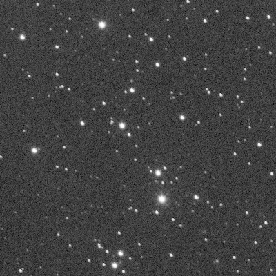
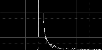
Both images are being shown with automatic screen stretch functions applied (STF AutoStretch). The MRS Gaussian noise estimates (NoiseEvaluation script) are, respectively for the top and bottom images:
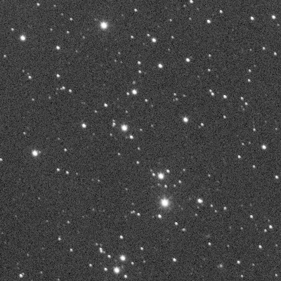
From these estimates, the bottom image seems to be about three times less noisy than the top image, so it should be weighted much more than the top image for integration (about 11 times more, assuming that SNR is proportional to the square root of the signal). Doesn't this seem to be contradictory to the visual appearance of both images? In fact, the bottom image is just a duplicate of the top image, multiplied by 0.3 with PixelMath (without rescaling), so both images have exactly the same signal and noise components, because other than the scaling operation, they are identical.
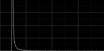
When integrating real images, similar situations to the one described above happen all the time due to different exposure times, sky conditions, sensor temperatures, and other acquisition factors. To compare noise estimates between different images, one has to take into account not only the noise values, but the scaling factors that must be applied to make the noise estimates statistically compatible. Besides noise estimation (and its associated image weighting criterion), pixel rejection also depends critically on estimators of location and scale. For example, with the images shown above, a pixel pertaining to the sky background in the top image would be ranked the same as a pixel on a relatively bright area in the bottom image, probably pertaining to a moderately bright star (compare the histograms to understand why this would happen).
In previous versions of the ImageIntegration tool, the median and average absolute deviation from the median were used as estimators of location and scale, respectively. The median is a robust estimator of location that works very well for linear images because the typical distribution of linear pixel values has a very strong central tendency. In other words, the main histogram peak in a linear image is very prominent. The average absolute deviation, on the other hand, is a nonrobust estimator of scale. As implemented in the ImageIntegration tool, the average absolute deviation is robustified by trimming too dark and too bright pixels, which excludes cold and hot pixels, as well as saturated pixels and bright spurious features (cosmics, etc). This approach has been working quite well so far. However, the efficiency and robustness of scale estimators is so crucial to many subtasks in the ImageIntegration process, that clearly some further research and development in this field has been necessary for some time.
I have tried to do my homework with the new version of ImageIntegration. The whole integration process is now more accurate and robust, and thanks to a new parameter, you can select a robust scale estimator to gain more control to squeeze the last bit of information from your data. The new parameter is readily available in the Image Integration section of the tool. Let's enumerate the estimators of scale available in the current version:
The selected scale estimator will be used in all subtasks requiring image scaling factors. This includes the noise evaluation image weighting routine, normalization in all pixel rejection algorithms, output normalization when a scaling option is selected (additive with scaling is now the default output normalization), and final noise estimation.
In general, the default IKSS estimator of scale works almost optimally in most cases. If you really want to get the most out of your data, you should at least make a few tries with IKSS, MAD and average absolute deviation. The goal is to maximize effective noise reduction (see the next section) while achieving a good outlier rejection.
Quality Assessment
When the evaluate noise option is selected, ImageIntegration performs a (scaled) noise evaluation task on the final integrated image, and compares these noise estimates with the original integrated frames in order to assess the quality of the integration. Without this final assessment, image integration is kind of a "faith-based" process, where one has no way to know if the achieved image is making justice to the data. This is contrary to the general philosophy of PixInsight. Bear in mind that the result of integration is the very starting point of your image, so knowing how good is it is of crucial importance.
Previous versions of ImageIntegration attempted to provide estimates of the signal-to-noise ratio (SNR) improvement. For example, we know that when we average N images, we get an SNR improvement equal to the square root of N. This is of course a theoretical upper limit, which we'll never achieve due to a number of adverse factors (we work with discrete signals, we reject some pixels, not all of the images have the same quality, etc). Unfortunately, estimating the relative SNR gain is not a trivial task, and the routines implemented in previous versions of the ImageIntegration tool were not as accurate as required. In some cases we have seen reported improvements slightly greater than the theoretical limit, which doesn't contribute to the confidence on these reports. We definitely need more accuracy.
The new version of ImageIntegration does not attempt to evaluate SNR increments. Instead, it provides accurate estimates of effective noise reduction. To understand how this works, consider the following images.
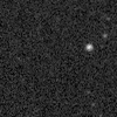
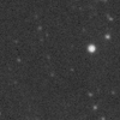
The image to the left is a crop of the reference frame of an integration set of 20 images. The right hand image is the same crop on the integrated result. Both linear images (the whole images, not the crops) are being shown with automatic screen stretch functions applied. We know that we can expect a maximum SNR improvement of 4.47 approximately (the square root of 20). The achieved improvement is self-evident by comparing the above images: the integrated result is much smoother than the original, and the higher SNR is also evident from many features that are clearly visible after integration, but barely detectable or invisible on the original.
This is a purely qualitative evaluation. Let's go a step forward in our analysis, and apply automatic screen stretch functions just to each crop (not to the whole images as before). As you know, the STF AutoStretch function is adaptive, so it computes stretch parameters based on statistical properties of each image. This is the result:
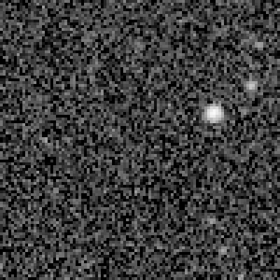
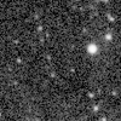
Clearly not as good as before. The integrated image still shows many dim stars that are barely visible on the original, but the background noise levels are now quite similar: the illusion of a smooth result has evanesced. To explain why this happens we need some quantitative analysis. If we compute robust estimates of dispersion and noise for these cropped images, we get the following values:
The first thing to note is that the standard deviation of the noise is quite similar to the corresponding scale estimate in each case (more in the original crop). This happens because these crops are dominated by the background of the image, where the noise also dominates over the signal. Now let's scale the integrated noise estimate with respect to the original. The scaling factor of the integrated crop with respect to the original crop is given by:
so the scaled noise estimate for the integrated crop is:
from which we can compute the effective noise reduction:
which represents about a 14% noise reduction. ImageIntegration has reported an effective noise reduction factor of 1.298 for the whole image in this case (integration of 20 images). Now you know why the noise in background areas is so difficult to remove, even after stacking a good bunch of images: as soon as you stretch the image, the noise comes back! Now you know also why robust scale estimators are so important.
This is how the new version of ImageIntegration evaluates the quality of an integration process. The good news is that this evaluation is much more accurate and robust than the SNR increments reported by previous versions. Don't let the low figures discourage you: they do not represent the improvement in SNR that your are achieving with your data, but the noise reduction achieved on low-signal regions, where noise estimates are very accurate and reliable as quality estimators.
So your goal when integrating a set of light frames is to achieve the maximum possible noise reduction, with the necessary rejection of outlier pixels. I hope this new version of the ImageIntegration tool will help you to get even more out of your data.
New ImageIntegration Cache
In previous versions of the ImageIntegration tool, the cache of statistical image properties is monolithic. This means that different statistical data items, such as estimates of scale and noise, are tied together: if you need just one of them, all of them have to be calculated, which is unnecessarily expensive.
The new version of ImageIntegration implements a granular cache, where all data items are independent each other. This greatly improves efficiency of the whole process because the data are computed strictly as they are required. Although I have made efforts to make the new cache compatible with old versions, as a safety procedure I strongly recommend you reset the ImageIntegration cache (click the arrow icon on the bottom control bar of the tool and click the Clear Memory Cache and Purge Persistent Cache buttons).
Availability of Source Code
The ImageIntegration tool has been released as an open-source product under the PixInsight Class Library License. The complete source code of the new version is now available as part of the latest PCL distribution, which we have also released today:
http://pixinsight.com/developer/pcl/download/PCL-02.00.04.0603-20130714.tar.gz
http://pixinsight.com/developer/pcl/download/PCL-02.00.04.0603-20130714.zip
References
[1] Rand R. Wilcox (2012), Introduction to Robust Estimation and Hypothesis Testing, 3rd Edition, Elsevier Inc., Section 3.12.
[2] P.J. Rousseeuw and C. Croux (1993), Alternatives to the Median Absolute Deviation, Journal of the American Statistical Association, Vol. 88, pp. 1273-1283.
A couple days ago I have released new versions of two essential PixInsight tools: ImageIntegration and StarAlignment. Both versions come with important new features and improvements, which I'll describe on this forum. In this post I'm going to focus on the new version of ImageIntegration.
New Scale Estimators
Statistical estimates of scale play an essential role in the image integration task. For example, comparisons of unscaled noise estimates from different images are meaningless. Consider the following two linear images and their histograms:
Both images are being shown with automatic screen stretch functions applied (STF AutoStretch). The MRS Gaussian noise estimates (NoiseEvaluation script) are, respectively for the top and bottom images:
top: 5.538?10-5
bottom: 1.661?10-5
bottom: 1.661?10-5
From these estimates, the bottom image seems to be about three times less noisy than the top image, so it should be weighted much more than the top image for integration (about 11 times more, assuming that SNR is proportional to the square root of the signal). Doesn't this seem to be contradictory to the visual appearance of both images? In fact, the bottom image is just a duplicate of the top image, multiplied by 0.3 with PixelMath (without rescaling), so both images have exactly the same signal and noise components, because other than the scaling operation, they are identical.
When integrating real images, similar situations to the one described above happen all the time due to different exposure times, sky conditions, sensor temperatures, and other acquisition factors. To compare noise estimates between different images, one has to take into account not only the noise values, but the scaling factors that must be applied to make the noise estimates statistically compatible. Besides noise estimation (and its associated image weighting criterion), pixel rejection also depends critically on estimators of location and scale. For example, with the images shown above, a pixel pertaining to the sky background in the top image would be ranked the same as a pixel on a relatively bright area in the bottom image, probably pertaining to a moderately bright star (compare the histograms to understand why this would happen).
In previous versions of the ImageIntegration tool, the median and average absolute deviation from the median were used as estimators of location and scale, respectively. The median is a robust estimator of location that works very well for linear images because the typical distribution of linear pixel values has a very strong central tendency. In other words, the main histogram peak in a linear image is very prominent. The average absolute deviation, on the other hand, is a nonrobust estimator of scale. As implemented in the ImageIntegration tool, the average absolute deviation is robustified by trimming too dark and too bright pixels, which excludes cold and hot pixels, as well as saturated pixels and bright spurious features (cosmics, etc). This approach has been working quite well so far. However, the efficiency and robustness of scale estimators is so crucial to many subtasks in the ImageIntegration process, that clearly some further research and development in this field has been necessary for some time.
I have tried to do my homework with the new version of ImageIntegration. The whole integration process is now more accurate and robust, and thanks to a new parameter, you can select a robust scale estimator to gain more control to squeeze the last bit of information from your data. The new parameter is readily available in the Image Integration section of the tool. Let's enumerate the estimators of scale available in the current version:
- As I have said above, the average absolute deviation from the median has been the default scale estimator used in previous versions of the ImageIntegration tool. It is robustified by trimming all pixel samples outside the [0.00002,0.99998] range, which excludes cold and hot pixels, as well as most saturated pixels and bright spurious features (cosmics, etc). Yet this is a nonrobust estimator (its breakdown point is zero), so its use is in general discouraged. It has one important advantage though: it is a rather sufficient estimator. Sufficiency of a statistical estimator refers to its ability to use all of the available sampled data to estimate its corresponding parameter. This explains why the average absolute deviation still works very well in some cases, and why it has been working well until now.
- The median absolute deviation from the median (MAD) is a very robust estimator of scale. Although it has the best possible breakdown point (50%), its efficiency for a normal distribution is rather low (37%). It tends to work better for images with large background areas (I'm using the term "background" here with a purely statistical meaning; it can be the sky but also a dominant background nebula, for example).
- The square root of the biweight midvariance[1] is a robust estimator of scale with a 50% breakdown point (as good as MAD) and high efficiency with respect to several distributions (about 86%).
- The square root of the percentage bend midvariance[1] is another robust estimator of scale with high efficiency (67%) and good resistance to outliers.
- Sn and Qn estimators of Rousseeuw and Croux.[2] The average deviation, MAD, biweight and bend midvariance estimators measure the variability of pixel sample values around the median. This makes sense for deep-sky images because the median closely represents the mean background of the image in most cases. However, these estimators work under the assumption that variations are symmetric with respect to the central value, which may not be quite true in many cases. The Sn and Qn scale estimators don't measure dispersion around a central value. They evaluate dispersion based on differences between pairs of data points, which makes them robust to asymmetric and skewed distributions. Sn and Qn are as robust to outliers as MAD, but their Gaussian efficiencies are higher (58% and 87%, respectively). The drawback of these estimators is that they are computationally expensive, especially the Qn estimator.
- The iterative k-sigma scale estimator (IKSS) implements a robust sigma-clipping routine based on the biweight midvariance. The idea is similar to M-estimators of location. From our tests, IKSS is as robust to outliers as MAD, and its Gaussian efficiency exceeds the 90%. This is the default estimator of scale in current versions of the ImageIntegration tool.
The selected scale estimator will be used in all subtasks requiring image scaling factors. This includes the noise evaluation image weighting routine, normalization in all pixel rejection algorithms, output normalization when a scaling option is selected (additive with scaling is now the default output normalization), and final noise estimation.
In general, the default IKSS estimator of scale works almost optimally in most cases. If you really want to get the most out of your data, you should at least make a few tries with IKSS, MAD and average absolute deviation. The goal is to maximize effective noise reduction (see the next section) while achieving a good outlier rejection.
Quality Assessment
When the evaluate noise option is selected, ImageIntegration performs a (scaled) noise evaluation task on the final integrated image, and compares these noise estimates with the original integrated frames in order to assess the quality of the integration. Without this final assessment, image integration is kind of a "faith-based" process, where one has no way to know if the achieved image is making justice to the data. This is contrary to the general philosophy of PixInsight. Bear in mind that the result of integration is the very starting point of your image, so knowing how good is it is of crucial importance.
Previous versions of ImageIntegration attempted to provide estimates of the signal-to-noise ratio (SNR) improvement. For example, we know that when we average N images, we get an SNR improvement equal to the square root of N. This is of course a theoretical upper limit, which we'll never achieve due to a number of adverse factors (we work with discrete signals, we reject some pixels, not all of the images have the same quality, etc). Unfortunately, estimating the relative SNR gain is not a trivial task, and the routines implemented in previous versions of the ImageIntegration tool were not as accurate as required. In some cases we have seen reported improvements slightly greater than the theoretical limit, which doesn't contribute to the confidence on these reports. We definitely need more accuracy.
The new version of ImageIntegration does not attempt to evaluate SNR increments. Instead, it provides accurate estimates of effective noise reduction. To understand how this works, consider the following images.
The image to the left is a crop of the reference frame of an integration set of 20 images. The right hand image is the same crop on the integrated result. Both linear images (the whole images, not the crops) are being shown with automatic screen stretch functions applied. We know that we can expect a maximum SNR improvement of 4.47 approximately (the square root of 20). The achieved improvement is self-evident by comparing the above images: the integrated result is much smoother than the original, and the higher SNR is also evident from many features that are clearly visible after integration, but barely detectable or invisible on the original.
This is a purely qualitative evaluation. Let's go a step forward in our analysis, and apply automatic screen stretch functions just to each crop (not to the whole images as before). As you know, the STF AutoStretch function is adaptive, so it computes stretch parameters based on statistical properties of each image. This is the result:
Clearly not as good as before. The integrated image still shows many dim stars that are barely visible on the original, but the background noise levels are now quite similar: the illusion of a smooth result has evanesced. To explain why this happens we need some quantitative analysis. If we compute robust estimates of dispersion and noise for these cropped images, we get the following values:
Original crop
scale = 6.4834?10-4
noise = 6.3535?10-4
Integrated crop
scale = 1.5207?10-4
noise = 1.3118?10-4
scale = 6.4834?10-4
noise = 6.3535?10-4
Integrated crop
scale = 1.5207?10-4
noise = 1.3118?10-4
The first thing to note is that the standard deviation of the noise is quite similar to the corresponding scale estimate in each case (more in the original crop). This happens because these crops are dominated by the background of the image, where the noise also dominates over the signal. Now let's scale the integrated noise estimate with respect to the original. The scaling factor of the integrated crop with respect to the original crop is given by:
scale = 6.4834?10-4 / 1.5207?10-4 = 4.2634
so the scaled noise estimate for the integrated crop is:
scaled noise = scale ? 1.3118?10-4 = 5.5928?10-4
from which we can compute the effective noise reduction:
noise reduction = 6.3535?10-4 / 5.5928?10-4 = 1.136
which represents about a 14% noise reduction. ImageIntegration has reported an effective noise reduction factor of 1.298 for the whole image in this case (integration of 20 images). Now you know why the noise in background areas is so difficult to remove, even after stacking a good bunch of images: as soon as you stretch the image, the noise comes back! Now you know also why robust scale estimators are so important.
This is how the new version of ImageIntegration evaluates the quality of an integration process. The good news is that this evaluation is much more accurate and robust than the SNR increments reported by previous versions. Don't let the low figures discourage you: they do not represent the improvement in SNR that your are achieving with your data, but the noise reduction achieved on low-signal regions, where noise estimates are very accurate and reliable as quality estimators.
So your goal when integrating a set of light frames is to achieve the maximum possible noise reduction, with the necessary rejection of outlier pixels. I hope this new version of the ImageIntegration tool will help you to get even more out of your data.
New ImageIntegration Cache
In previous versions of the ImageIntegration tool, the cache of statistical image properties is monolithic. This means that different statistical data items, such as estimates of scale and noise, are tied together: if you need just one of them, all of them have to be calculated, which is unnecessarily expensive.
The new version of ImageIntegration implements a granular cache, where all data items are independent each other. This greatly improves efficiency of the whole process because the data are computed strictly as they are required. Although I have made efforts to make the new cache compatible with old versions, as a safety procedure I strongly recommend you reset the ImageIntegration cache (click the arrow icon on the bottom control bar of the tool and click the Clear Memory Cache and Purge Persistent Cache buttons).
Availability of Source Code
The ImageIntegration tool has been released as an open-source product under the PixInsight Class Library License. The complete source code of the new version is now available as part of the latest PCL distribution, which we have also released today:
http://pixinsight.com/developer/pcl/download/PCL-02.00.04.0603-20130714.tar.gz
http://pixinsight.com/developer/pcl/download/PCL-02.00.04.0603-20130714.zip
References
[1] Rand R. Wilcox (2012), Introduction to Robust Estimation and Hypothesis Testing, 3rd Edition, Elsevier Inc., Section 3.12.
[2] P.J. Rousseeuw and C. Croux (1993), Alternatives to the Median Absolute Deviation, Journal of the American Statistical Association, Vol. 88, pp. 1273-1283.
")