Messier 31 H-alpha Processing Notes
By Vicent Peris (PTeam/OAUV) and Alicia Lozano
Published February 25, 2022
Introduction
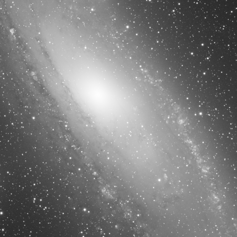
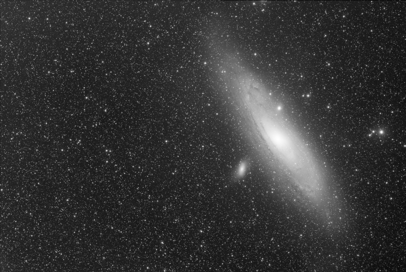
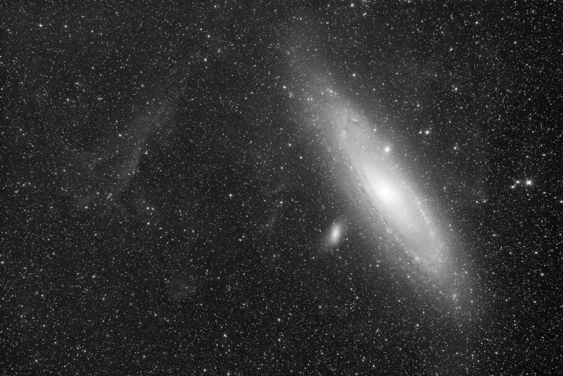
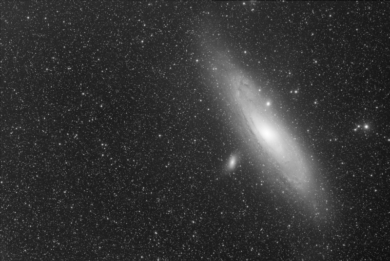
Sometimes you see in your mind your already finished picture even before starting to shoot it. The original idea to produce the Andromeda galaxy picture that we have published in the PixInsight Gallery comes from a picture of the core of the same galaxy Vicent produced some years ago at Calar Alto observatory with the 3.5 meter telescope:

© Vicent Peris (OAUV), Gilles Bergond (CAHA), Jack Harvey (SSRO), CAHA, Fundación Descubre, OAUV, DSA.
This image uses [O-III] and H-alpha filters to enhance line-emitting objects. To adequately process the image, it is necessary to remove the continuum emission from the narrowband filter images—we'll talk about this in the Continuum Subtraction section. In this way we isolate the pure oxygen and hydrogen light emissions. Only then it is possible to unveil the gaseous spiral structure right to the galaxy nucleus. Our idea was to produce this artwork by using this technique to undress the galaxy and bring out its entire delicate geometry. This galactic skeleton would then fall into the thin clouds of hydrogen at the bottom of the picture, like a model dropping his/her clothes on the floor.
Mouse over:
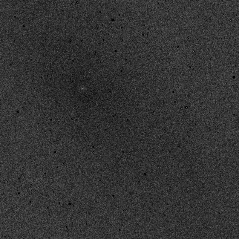
The original narrowband H-alpha image.
The narrowband H-alpha after removing the continuum light emission.
In this article we'll focus on the use of some of the preprocessing tools available in PixInsight 1.8.9, as well as on the generation of a picture showing the pure hydrogen light emission.
Preprocessing Notes
Dataset
The dataset comprises images acquired with H-alpha and red filters. The red exposures are acquired only to subtract the continuum emission from the narrowband image, in order to show the pure hydrogen emission. Two short-exposure subsets of red-filtered images were also needed for the bright galaxy nuclei and to restore the stars that were degraded by the continuum subtraction operation.
The H-alpha subset, acquired with a QHY600L (60 megapixels and 3.76 μm pixels) is a highly heterogeneous set of images for the following reasons:
- They were acquired at altitudes ranging from the zenith down to 20°.
- We acquired data in all the available nights during November and December, so there are images acquired under very different Moon conditions, even some nights with the full Moon at 30° from the galaxy.
- Some nights had also thin cirrus clouds.
- Seeing conditions were highly variable. Some groups of images are affected by turbulence even at 2 arcseconds per pixel.
- This was a new camera with a new, custom-made adapter. The camera was not completely orthogonal to the optical axis, so the stars are slightly defocused towards the right side of the image.
Subframe rejection and weighting is an important topic. However, how we reject and weight the images is highly dependent on the object and the goal of the picture. In this case, our primary goal was to obtain as much signal as possible on the faint background nebulae, so we made two delicate decisions to preprocess this subset. First, we weighted the images based exclusively on the noise of each subframe; then, we also decided to include subframes with sligh defocus, bad guiding and poor seeing. On the other hand, we discarded images with cirrus or too strong gradients, which would negatively affect the signal and reliability of the background nebulae. The resulting H-alpha master has slightly increased star sizes but it has as much signal as possible from these faint structures. How we recover the stars and their sharpness is explained in the Star Restoration section.
The primary red filter subset is comprised of 600-second exposures shot with a Finger Lakes Microline ML16200. This camera has a 16-megapixel CCD sensor with 6 μm pixels. We should remark two things about this subset:
- Having bigger pixels, we used as registration reference the H-alpha master coming from the QHY600 camera and used drizzle x1, which resulted in a big improvement in resolution and data reliability. By registering the 6-μm pixels to 3.76-μm pixels, it's like using drizzle at x1.6.
- This camera has a smaller sensor, so we needed to do a two-panel mosaic to cover the entire field of view of the QHY600. Since the QHY600 camera image works as the registration reference, we don't need to assemble an astrometry-based mosaic; the two panels simply adapt to the geometric distortions of the reference.
- We needed a long exposure time in the red filter because we were going to use this image to subtract the continuum emission from the H-alpha image. Having a poor quality red image would contaminate with noise our pristine H-alpha image. Therefore, we shot 7 hours of exposure time per panel.
Last, we needed short exposures with the red filter, which were acquired with the QHY600 camera:
- A 30×30-second exposure set was acquired to perform an HDR composition over the nuclei of M31 and M32.
- A 50×10-second exposure set—of which we only used 14—was also acquired to recover the stars from the degradation they suffered in the processing. We talk extensively about this in the Star Restoration section.
Preprocessing Workflow
Below you can see the entire preprocessing workflow applied to preprocess all image subsets. At the end of this stage we have three master images:
- The H-alpha master.
- The HDR red master, used to subtract the continuum light from the H-alpha master.
- The short, 10-second exposure red master, used to restore the stars in the continuum-subtracted image.
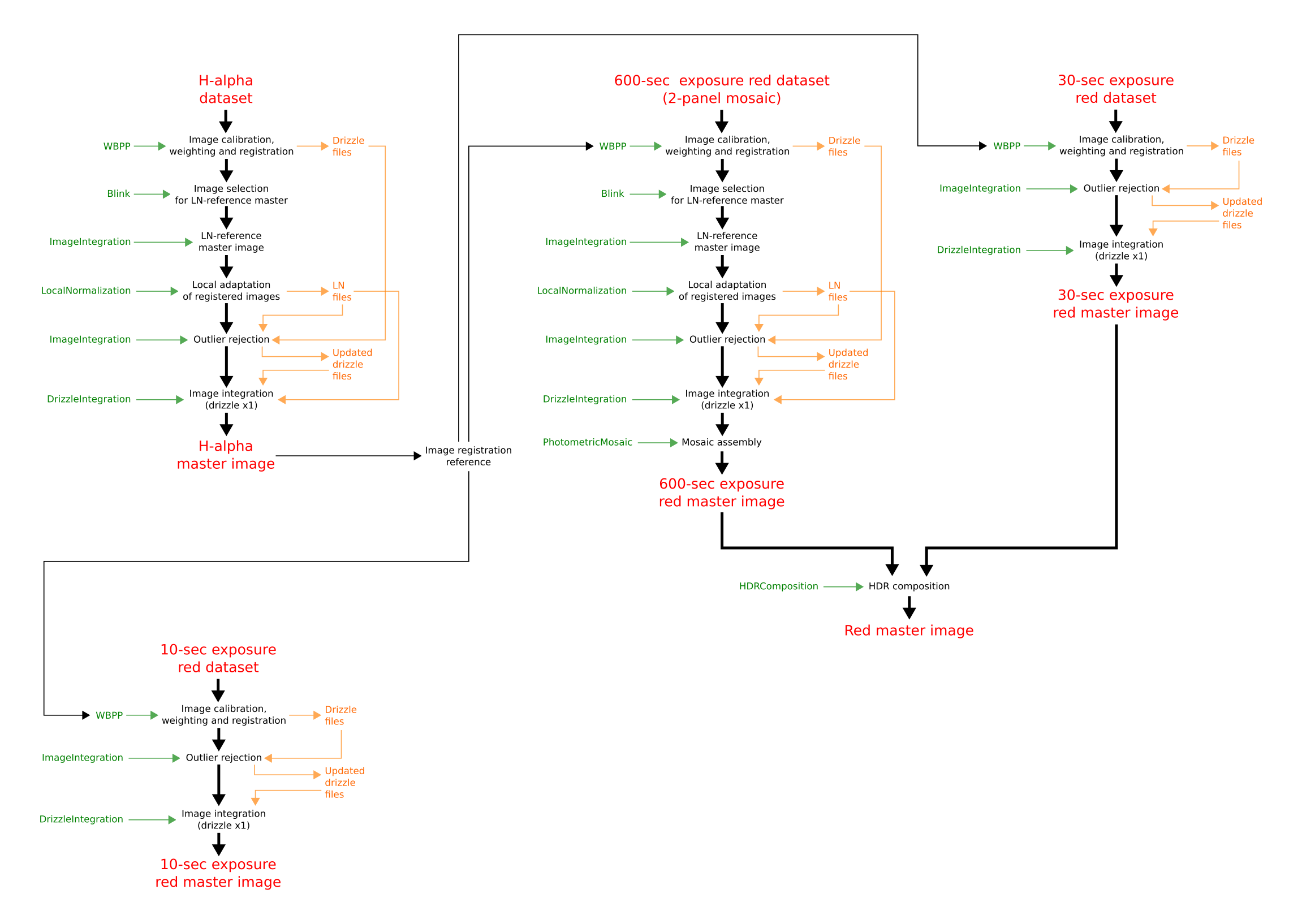
Click on the image to see the diagram at full scale.
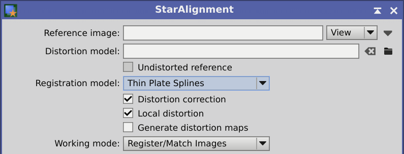
There are a few specific points to point out in this workflow. First of all, we use the H-alpha master image as registration reference for the three red image subsets. This provides a high quality registration reference for those images, but it also lets us assemble the two-panel mosaic of the long-exposure red images without the use of astrometry tools. The two panels are simply registered to the H-alpha master and they reproduce the focal plane distorsions of that image, since we configure the WeightedBatchPreprocessing script for distortion correction in the light image registration section. If you run separately StarAlignment, you should modify these settings to adapt the geometry of the target images to the reference:
As you can see, we use the LocalNormalization tool with a master image as normalization reference. This increases the reliability of the final image because all of the normalized subframes will inherit the very-large-scale noise of the reference image. Therefore, having a high-quality reference image will reduce the impact of this noise in the resulting master image. To generate the LocalNormalization reference master, we manually selected the best subframes using Blink. This has been completely automated in version 2.4.0 of the WeightedBatchPreprocessing script, which is available in PixInsight 1.8.9. We'll later show how the photometry evaluation of LocalNormalization affects the image integration process to help having the best possible rejection of outliers in the image set.
The use of drizzle throughout the preprocessing stage is imperative, especially for the red images coming from the Finger Lakes camera. We'll show later how drizzle completely eliminates the interpolation artifacts created when resampling the 6-μm image to the 3.76-μm ones.
We, as astrophotographers, are always on the search of the purest possible image from which to start our postprocessing work. Having a preprocessing workflow with completely integrated image weighting, local normalization, efficient outlier rejection and drizzle techniques is fundamental because each of these techniques have big impact on the reliability of the information in the resulting master image.
Photometry-based Image Scaling with LocalNormalization
In astrophotography, the light from the objects always sits on top of the background sky light. This defines how we adjust the brightness of a night sky image. While the sky brightness is an additive contribution to the image, when we want to fit the brightness of the objects between two images we need to find a multiplicative factor. The appropriate additive and multiplicative factors will adapt the sky background level and the light intensity of the objects between both images, making them statistically compatible along the crucial preprocessing steps.
While finding the additive component is relatively easy, finding the multiplicative factor requires more sophistication. Statistical estimators of scale applied globally to the entire images usualy don't work because in deep-sky astrophotography there is always a large contribution of the noise at that global scales. Fortunately, we always have point light sources in our images: the stars. By measuring the light intensity of the same stars in both images, we can calculate accurately the scaling factor required to adapt one image to the other.
The faster way to measure the brightness of a star is by the use of aperture photometry, which measures all the light contained in a box centered on each star. In a linear image, all the stars have the same size independently of their brightness, so the first requirement of aperture photometry is to use the same box size where to measure the light for all the stars over the entire image. In this way we can be sure to be measuring the same fraction of the light in every star.
However, in the real world, not all of the stars have the same shape and size throughout the image. No matter how well collimated is a telescope, when we measure the PSF in the image we'll always find variations in shape and size on different areas of the focal plane. To tackle this problem, the updated LocalNormalization tool available since PixInsight 1.8.9 uses a hybrid PSF and aperture photometry methodology, where the sizes and shapes of the measuring regions are defined adaptively by fitting a different point-spread function to each detected source.
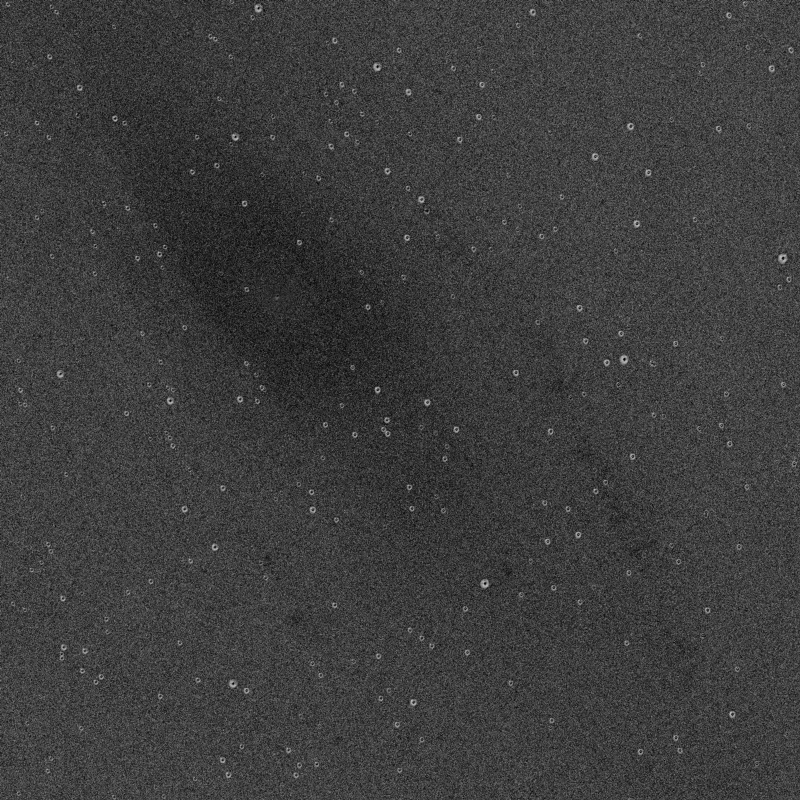
In our image the camera had some tilt, so the stars were definitely bigger on the right side. The AberrationSpotter script shows this tilt very well in the H-alpha master image:
We can also render FWHM and eccentricity maps of the stars in the image with the FWHMEccentricity script:
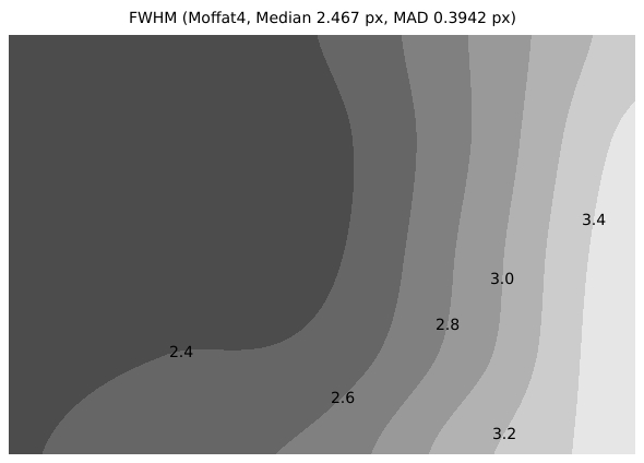
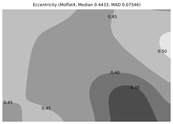
Using the same measuring box all over the entire image would cause a systematic error in the image set because we would be measuring a lower fraction of light of the stars towards the right side of the image. Thus, by using varying measuring regions defined by PSF fits in LocalNormalization, we increase the reliability of the measurements, as we adapt them to each star.
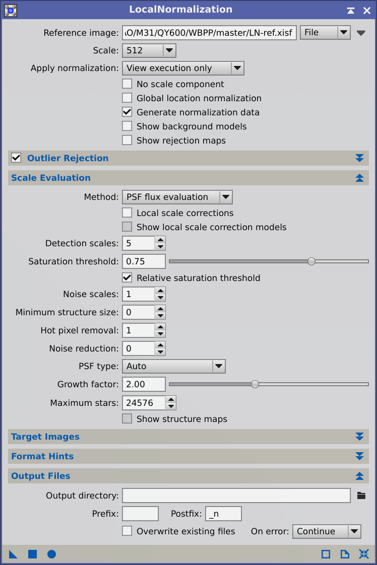
For this dataset, we used LocalNormalization to correct for variations in the local background. We also corrected the signal intensity globally in each image, since the local scaling feature is still under development (although you can use it for experimentation purposes). We used the default 512-pixel normalization scale. We also increased the Growth Factor parameter value to 2, in order to enlarge the measurement area around each star, which showed to improve the scale estimates. Below you can see the applied LocalNormalization settings:
One of the goals of LocalNormalization is to compatibilize the entire image set to optimize rejection of outliers in the image integration process. So testing the outlier rejection will indicate how well LocalNormalization is performing. We ran LocalNormalization two times, one with global scale adaptation and another without scaling (only the additive factor from the sky background).
To test the subframe adaptation, we ran ImageIntegration with the Linear Fit Clipping rejection algorithm. We used a highly stringent rejection by lowering the sigma limits to 5 on both sides (for a 300-subframe image set we need to increase the rejection limit to 8-9 sigmas). This produces a too high pixel rejection but shows very well how well the adaptation is working, since a disagreement in the light intensity between the subframes will lead to a rejection of significant image structures. Below we have the rejection maps coming out of the integration using LocalNormalization to normalize only the additive component. We were correcting this component locally using a scale of 512 pixels.
Below we compare the rejection maps by running LocalNormalization with and without scaling. First, the rejection high maps:
And the rejection low maps:
Without using scaling factors, the rejection is completely polarized towards the low end on the galaxy core, which causes a severe rejection in this area (look at the bright core in the low rejection map). This rejection can cause problems in the master image, like an important increase in the noise level on this area. By using the scale correction in LocalNormalization, the rejection is much more uniform in both sides of the pixel distribution, showing only a slightly bright galaxy nucleus on the rejection low map (which will probably be completely corrected once we finish the development of local scale normalization).
It is important to note that the outer halos of the stars are rejected in both runs because we have integrated subframes with sligh defocus and bad seeing conditions.
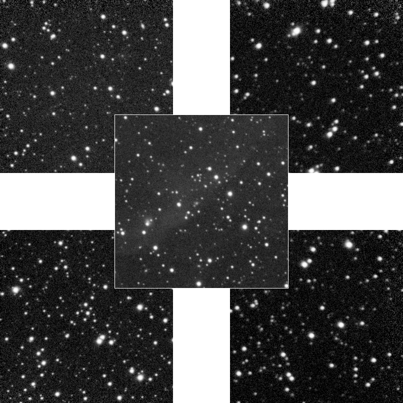
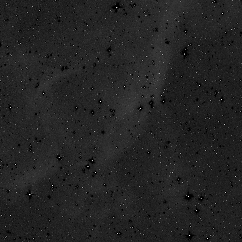
In the preprocessing workflow of our latest pictures we have included the generation of an additional master light coming from the best images in the dataset. This master acts as the reference image in the LocalNormalization tool. To select those images, we loaded the calibrated and registered subframes into the Blink tool and looked for the frames with less gradients and stronger signal. We followed this approach in our search for a master light with the best possible information reliability. Even at a scale of 512 pixels, noise contribution is more than significant, and basing the normalization process on a single frame as reference can affect the reliability of the large-scale nebular structures. Here you can see a comparison of the 512-pixel structures in five individual H-alpha light frames, each being a 10-minute exposure:
As you can see, the shapes of the background nebulae change even at this extremely large scale. The only way to reassure a minimum of reliability on those nebulae is to integrate multiple subframes into a master light as reference for the LocalNormalization process. For this image, we generated this normalization master with 30 subframes, so we used about a 10% of the total exposure time (5 hours). Here you can see the 512-pixel structures of this normalization master:
When you integrate all of these frames, you'll always get some gradients, even if you integrate the best images. In this image there is a soft dark gradient towards the right side, but it is easily corrected with the DynamicBackgroundExtraction (DBE) tool. What is important in this master is that those large structures have been averaged from 30 individual frames.
In PixInsight 1.8.9 this procedure has been automated: the WeightedBatchPreprocessing script will automatically select a subset of the best frames, based on PSF Signal Weight estimates, and will create this additional master light for the local normalization process. Although it is wonderful to automate this feature and the WBPP will work well in most cases, for an accurate work we recommend generating this master by hand using the SubframeSelector tool and reviewing the selected image subset visually with Blink.
Drizzle Results
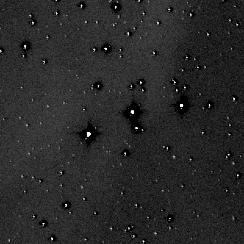
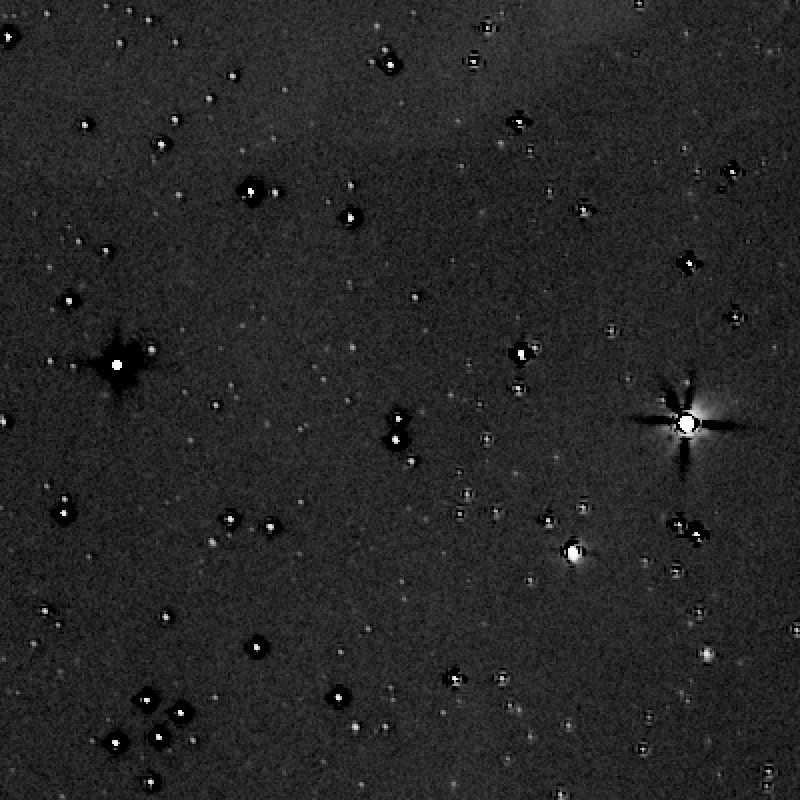
Drizzle has been very helpful in this image and, generally speaking, we strongly recommend the use of this technique in every image. The improvement in the long-exposure red images was dramatic because the upsampling needed to register them to the higher resolution H-alpha master was creating strong artifacts around the stars. The use of drizzle avoids this upsampling, which results in an artifact-free image:
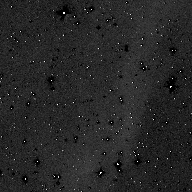
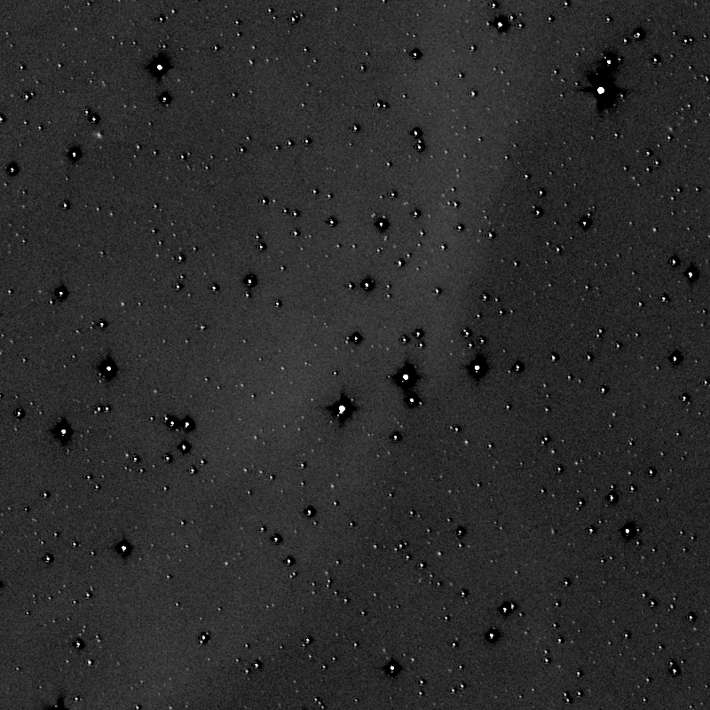
Accurate pixel interpolation algorithms tend to create a sharpening effect in the resampled image, thus causing the artifacts above. Some stars have dark ringing and some others have cross-like artifacts. The background tends to be noisier as well without drizzle. Those cross-like artifacts are also visible in the 10-second exposure master:
Mouse over:
Master 10-second exposure red image without drizzle.
Master 10-second exposure red image with drizzle.
Though the use of drizzle results in slightly bigger stars (since, as noted above, any precise resampling algorithm causes a sharpening effect), what is really important here is the fact that we have an artifact-free image.
It is important to point out that all of these artifacts are unavoidable when interpolation algorithms are applied for upsampling. We strongly recommend the use of the normalization and drizzle workflows that are implemented in the standard distribution of PixInsight, since this will let us have the best possible result in the master image. Since PixInsight 1.8.9 all of these steps are completely automated and this implementation will offer to you, in most cases, an automated master generation that will be close to the best result you can get manually.
Continuum Subtraction
Not everything in this image comes from the hydrogen emission. In a narrowband filter we still have light coming from light sources emitting a continuous spectrum; mostly stars in this image. This can be better understood by looking at a typical narrowband filter transmission curve:
While the filter keeps nearly 100% of light transmission at the desired emission line, it cuts the off-band transmission. And the narrower filter will do it more efficiently since the cut-off of the tranmission curve will be closer to the emission line. But this curve will always have two wings of transmission at both sides of the line, meaning that some light from the continuum-emitting objects will pass through the filter. The narrower these wings are, the dimmer will be the stars compared to the nebulae. So we should keep in mind that there is no narrowband filter where the continuum emission is completely blocked.
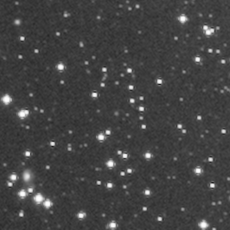
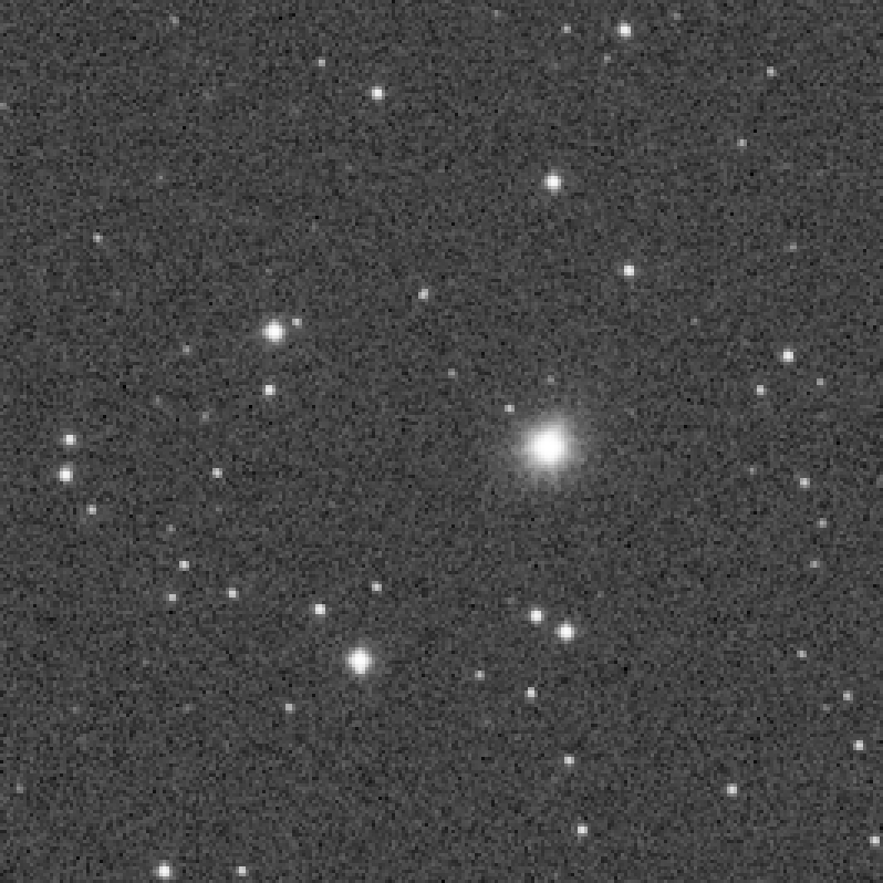
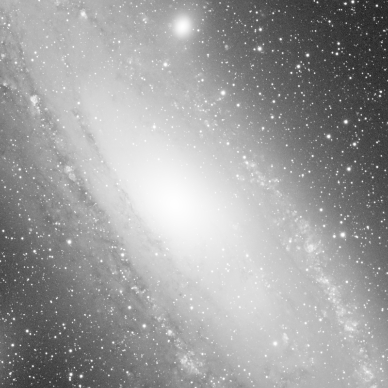
How much does this affect our M31 image? First, let's compare the broadband red and the narrowband, 5-nm H-alpha images:
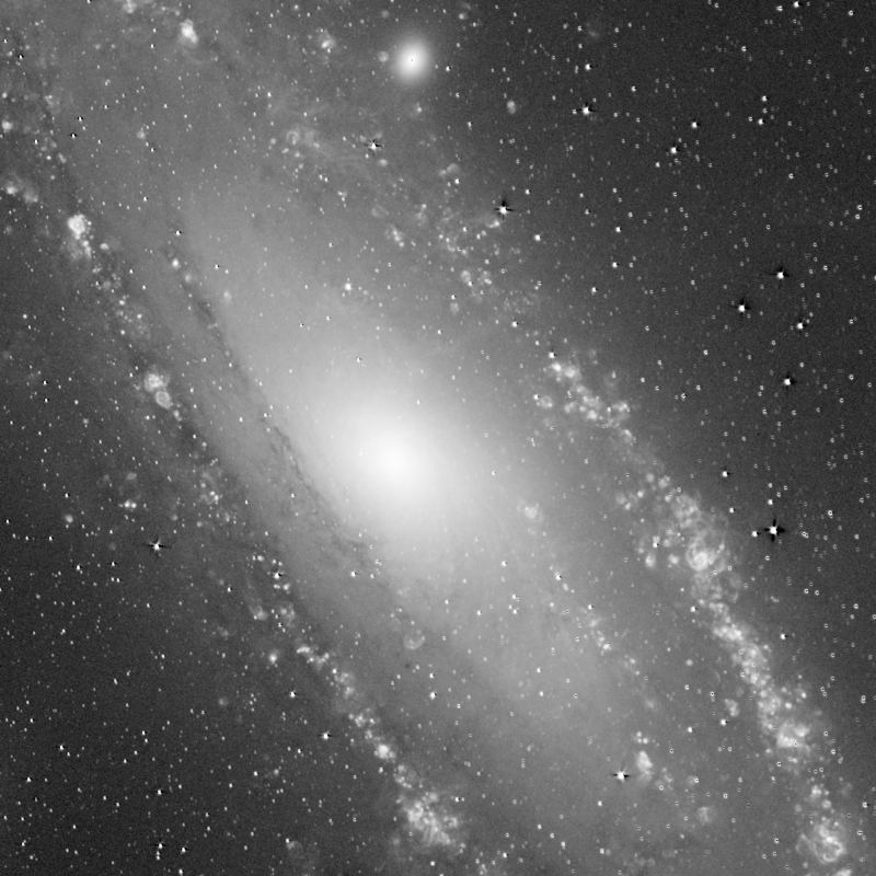
We could think that a 5-nm filter produces a very good isolation of the nebulae from the star population in the galaxy, but how much does the continuum emission contribute to the narrowband image? The comparison between the original H-alpha image and the continuum-cleaned one produces a dramatic change in the galaxy:
The effect of cleaning the H-alpha image from the continuum light is especially visible in the areas around the galaxy core, where the suppression of the stellar population lets us dig into the spiral structure of the hydrogen clouds:
We can conclude that there is a large amount of information coming from continuum emitting light sources in this image. If we look carefully at the comparisons above, we'll see that even some of the diffuse structures around the galaxy belong to its outer stellar halo, and not to hydrogen nebulae.
Now put this in the context of a color image. If we want to produce a color image of this field with hydrogen emission enhancement, it is mandatory to subtract the continuum light inside the H-alpha image. Not subtracting this continuum component in the narrowband image will seriously compromise the documentary value of a color picture, since we'll be enhancing red color areas that are not nebulae but stellar halos of the galaxy.
The process of subtracting the continuum light in the narrowband image is done with PixelMath. We multiply the R image by a small factor (k) to fit the starlight intensity of the red filter in the H-alpha filter:
Ha - (R - med(R)) * k
In this equation, we subtract the median value of R, which is representative of the background sky level, to maintain the current background sky level of the H-alpha image. Finding the k factor can be easily done by trial and error, since a too high value will start to create dark structures in the areas where the stellar contribution is higher. Here you have the result of performing the continuum subtraction with several k values:
Please note that this value does not represent the ratio of bandwidths between the filters, since there are additional conditioning factors to take into account. Some of them, like the change in atmospheric transparency, are always random, so we'll always need to find the right scaling factor of the R image. Moreover, in this data set the broad and narrowband images come from different cameras with different gains and pixel sizes. Anyway, the scaling factor will presumably be always small.
A long exposure time in the red filter is needed to avoid contaminating the H-alpha image with noise in the continuum subtraction operation. We shot 7 hours per panel. We tried to subtract shorter exposures but we did not achieve a good result by denoising the red image with any of the denoising techniques available, since the low surface brightness H-alpha nebulae are very delicate and the noise reduction affects the reliability of the results.
Star Restoration
The drawback of the continuum subtraction technique described above is that the stars will always be contaminated by artifacts, because it is impossible to have two images with exactly the same PSF. Those artifacts always affect the areas around stars. Thus, the critical part of the processing of this image is to restore the stars to an artifact-free shape.
Our goal in this image is to show the pure H-alpha line emission, so ideally this picture would not have any star inside. But, being impossible to completely subtract the stars from the image, we chose to show them at only an 8% of their original brightness. This is done by adding back the stars multiplied by a factor of 0.08 through a star mask. So we apply this formula in PixelMath:
(R - med(R)) * 0.3 * 0.08 + med(Ha)
Below is the corresponding PixelMath window. The process is again applied to the H-alpha image through a star mask:
However, a simple superimposition of the R stars over the H-alpha image will never work because they are two completely different, and hence incompatible images. Here we can see the result of recovering the brightest stars with the R image:
Mouse over:
Original continuum-subtracted, H-alpha image.
Continuum-subtracted, H-alpha image with superimposed R stars scaled at 8%.
Star mask.
The superimposed stars through the star mask are shown with dark or bright halos, depending on how the local brightness of the R image compares to the H-alpha one. To overcome this problem, we applied a technique that Vicent has been applying to his images during many years, called adaptive multiscale structure transfer (AMST). In its most basic form (which works well here because the image has a small dynamic range), the technique uses a formula with a simple subtraction and addition of large-scale components:
a - a_LS + b_LS
The idea behind this simple formula is transferring small-scale structures from one image to another, by placing them on top of the large-scale components of the target image. So, to apply this technique, we work with four different images:
Mouse over:
The R image, with "R" identifier.
The large-scale components of the R image, with "R_LS" identifier.
The continuum-cleaned, H-alpha image, with "Ha" identifier.
The large-scale components of the continuum-cleaned, H-alpha image, with "Ha_LS" identifier.
This is the PixelMath dialog, which we'll apply to the H-alpha image through a star mask:
In this PixelMath instance, the first multiplier is the red image scaling factor that adapts the brightness of the stars to those in the H-alpha image, as previously seen. The second factor multiplies then the brightness of the stars to achieve the desired 8%. This process removes the large-scale components of the image whose small-scale structures are going to be transferred, and those small-scale structures are placed on top of the large-scale components of the image that receives the structures. However, when we add the stars multiplied by this small factor, we also multiply the noise by the same factor. The result is that we have stars surrounded by noise-free halos. This can be easily seen in this view at 1:1 zoom level:
Our goal, as usual, is to assemble an image where all of the components fit together. A quick and simple solution would be to add noise to the image with the NoiseGenerator tool through the star masks, to equalize noise levels throughout the image. This worked quite well and our first version of the picture was indeed produced with this trick. But this would, in our opinion, compromise the documentary value of the picture and the ethical integrity of our work. This is a particularly critical decision considering that, after applying all the star masks that we need to correct all the stars in the image, we would be filling almost the entire image with synthetic noise:
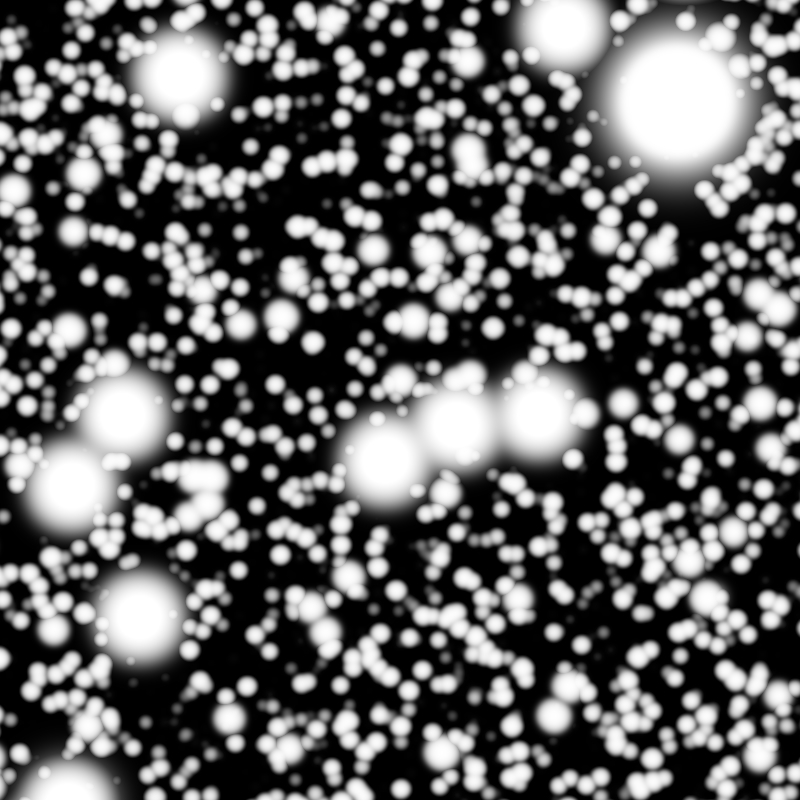
An addition of all the star masks used shows that they fill almost the entire image.
Therefore, we tried to find a more ethical approach to restore the stars in the image. Ideally, we would need to have a red image where, once multiplied by 0.08, its noise level is the same as the one in the H-alpha image. That is to say that we would need, in fact, a noisier red master image where to get the stars from. One option would be to use the short, 30-second red exposures to restore the stars, since this master image has a much shorter exposure time and hence a much higher noise level. But our experiments showed that even the 30×30-second red master image had a too high signal to noise ratio. You can see below a comparison between the restored stars by using the long exposures and the 30-second exposures in the red filter:

Mouse over:
Without star restoration.
Star restoration with 42×600-second red master.
Star restoration with 30×30-second red master.
Star mask used in the process.
The real problem here is that we are using drizzle, so we need a minimum amount of subframes for the short exposure red image. We cannot generate a good short exposure master red image using drizzle and only 5-6 subframes, since we could have artifacts on the stars. We then decided to shoot a sequence of 10-second exposures with the red filter. Once preprocessed, we calculated the number of 10-second subframes we needed to integrate by comparing the noise level in a single 10-second subframe to the master H-alpha image.
To calculate the number of subframes needed to match the noise level of the H-alpha image, we measured the noise level in a small background area of both the continuum-subtracted H-alpha image and a single 10-second exposure. We simply compared the MAD estimates in these areas:
- Continuum-subtracted H-alpha image: MAD = 0.0000126.
- Single 10-second red exposure, after scaling: MAD = 0.0000452.
The noise measurement in the 10-second exposure is done after scaling it to an 8% of the star brightness in the H-alpha image. If we square the ratio between both noise levels, we'll know how many 10-second subframes we need to integrate to have compatible noise levels between both masters:
(0.0000452 / 0.0000126)^2 = 12.87
So we need to integrate 13 subframes. We added an additional subframe to compensate for the loss of signal-to-noise ratio due to the pixel rejection. Therefore, we generated a 14×10-second exposure red master image. This way we would fit the noise levels once the short exposure master is scaled at the 8% of the starlight intensity in the H-alpha image:
Mouse over:
Without star restoration.
Star restoration with 42×600-second red master.
Star restoration with 30×30-second red master.
Star restoration with 14×10-second red master.
Star mask used in the process.
This solution has an additional advantage: the stars in the image are as sharp as possible, since no guiding corrections were used and there isn't any focus drift during the sequence.
By using this master red image, both images fit together like if they had always been only one. Ironically, the documentary integrity of the 51-hour H-alpha image was achieved by the use of a 140-second exposure in the red filter, but this logical thinking builds a picture where each element assembles to the others perfectly. Let's remember which is the complete process that restores the stars:
Mouse over:
Original, continuum-subtracted H-alpha image.
Simple superimposition of the long-exposure red master.
Superimposition of the long-exposure red master by using AMST.
Superimposition of the 14×10-second red master by using AMST.
Star mask used in the process.
In these figures we are restoring only the brighter stars, but this picture needed 11 different star masks to completely restore all of the stars in the image. Here we can see the result of the entire restoration process:
Mouse over:
Original, continuum-subtracted H-alpha image.
Image after the star restoration processes.
Addition of all the star masks used in the processes.
Conclusion
There are two important conclusions to draw from the work with this image. First, this data set has been a very good test bench for the improvements that we are implementing in our preprocessing tools, which are available in PixInsight since version 1.8.9. We do think that we have right now a state-of-the-art preprocessing pipeline, and we hope you'll enjoy it.
On the other hand, this image is very representative of our philosophy of the art and technique of astrophotography. In the first version of this picture we added synthetic noise around the stars. This works really great... until you realize that you are making up almost the entire image. Producing a honest image requires hard work sometimes, as well as an active search for unique solutions. But then you end up with a picture and a work that you are proud of.