Comet C/2022 E3 (ZTF)
Processing Notes

By Vicent Peris (PTeam/OAUV) and Alicia Lozano
Published February 7, 2023

---

Introduction

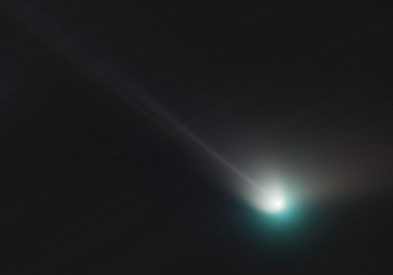
Comet C/2022 E3 (ZTF) has been very close to Earth. This poses additional problems to imagers since the comet needs to be tracked during its high-speed journey among the stars. In its closest approach, even short exposures of 2-minute length showed trailing stars:

PixInsight's current toolkit is not designed to detect and measure this kind of trail. Instead, it always works on reasonably round PSFs. Knowing in advance that ZTF would become a high-speed comet, we decided to update the CometAlignment tool to be able to work in a workflow where there are no reference stars.

In this article we also describe an observational methodology to apply a photometric color calibration to high-speed comets.

Using CometAlignment on Calibrated Subframes

The grayscale image animations we present in the video of this comet were acquired by blindly tracking the comet using its orbital elements and a Planewave L-350 mount. Instead of tracking the stars, the mount followed the comet's trajectory. Since the comet was moving at more than 15"/minute, our 2-minute exposures had star trails about 45 pixels long. The StarAlignment process has not been designed to work with this kind of PSFs, so CometAlignment cannot be applied to the images registered to the stars. Therefore, working with the calibrated-only images is the only way to align the comet.

The comet's path is a straight line when the stars have been aligned in a subframe set. But, if we want to locate the comet in an image set that has been only calibrated, we need to be able to adapt to non-linear trajectories. In this image set, the actual comet position is subject to any kind of positional errors, like mount and tube flexures. This means that the comet's path will never be a straight line but a curved and irregular one. CometAlignment has been recently updated for this reason.

Now we can configure multiple fixed points of the comet's path in CometAlignment. To add a new fixed path point, we double-click on any of the images in the list; CometAlignment will open the image, and then we'll be able to click on the comet's nucleus. Since we had long exposure sets of around 300 subframes per night, we decided to indicate the comet's position in 50-image steps.

With this working methodology, CometAlignment can fail if there is a significant movement in the image set. Therefore, we recommend setting the comet's position in the first and last images and then placing intermediate fixed positions. In this way, CometAlignment will draw an initial comet trajectory calculated from the two closest fixed positions when we open any intermediate images. If that position is very far from the actual comet's position, that's because you have a significant movement near that image.

If we work on the calibrated images, we always recommend generating the comet path mask to check if the comet's position has been well detected in all the subframes. Here we have the comet path in the image set from January 30:

This image also gives us valuable information. In this case, to the left side of the comet path, two positions clearly depart from the main curve. This is because the comet was passing very close to a bright star:

In this case, we can simply load the first image of the sequence and the two affected images in CometAlignment again. We can then indicate the precise comet's position in the three images to have them correctly registered.

Automated Image Processing

The time lapses presented in the video have been entirely processed in PixInsight using image containers. Here you have some advice to plan a uniform processing workflow for an image sequence:

• We want a very stable processing workflow that will produce uniform processing of the entire image sequence.
• First, use an image container with a few images representative of the entire sequence. Perform a quick test of the processing workflow to refine it.
• If we want to apply the same stretching to all the images, it's better to equalize the background sky to a specific level. This can be done easily with PixelMath. Then, use the same histogram transformation for all the images.
• The step above is mandatory if we want to apply curves after the stretching. The same curve will always need the same sky background level to work properly on the image.
• Some multiscale processes may not be stable enough in some cases. One example is HDRMT. In these sequences, HDRMT led to varying brightness of the comet nucleus. Instead, it's better to use simpler algorithms like curves or LHE to control the contrast in the image.

The processes applied to the images are as follows:

First, we equalize the sky background level to 0.01 with PixelMath:

Then, the image is stretched using HistogramTransformation:

Please remember that we apply exactly the same transformation to every image in the sequence. After this step, we increase the contrast between the background sky and the ionic tail with CurvesTransformation:

The last processing step is to apply a gentle LocalHistogramEqualization process to enrich the structures in the tail.:

Above complexity or effectivity, this workflow provides an entirely stable result that is critical to have a congruent time-lapse of the comet. These processes can be applied to every single frame. But, to better visualize the faint ionic tail, we decided to increase the signal-to-noise ratio of each image by designing a rolling image integration script. This script applied a rolling integration in blocks of 5 images to the entire image sequences. This means that the first frame in the video is the integration of frames 1 to 5, the second frame is the integration of 2 to 6, and so on. Below you can see the ImageIntegration process we used in this script:

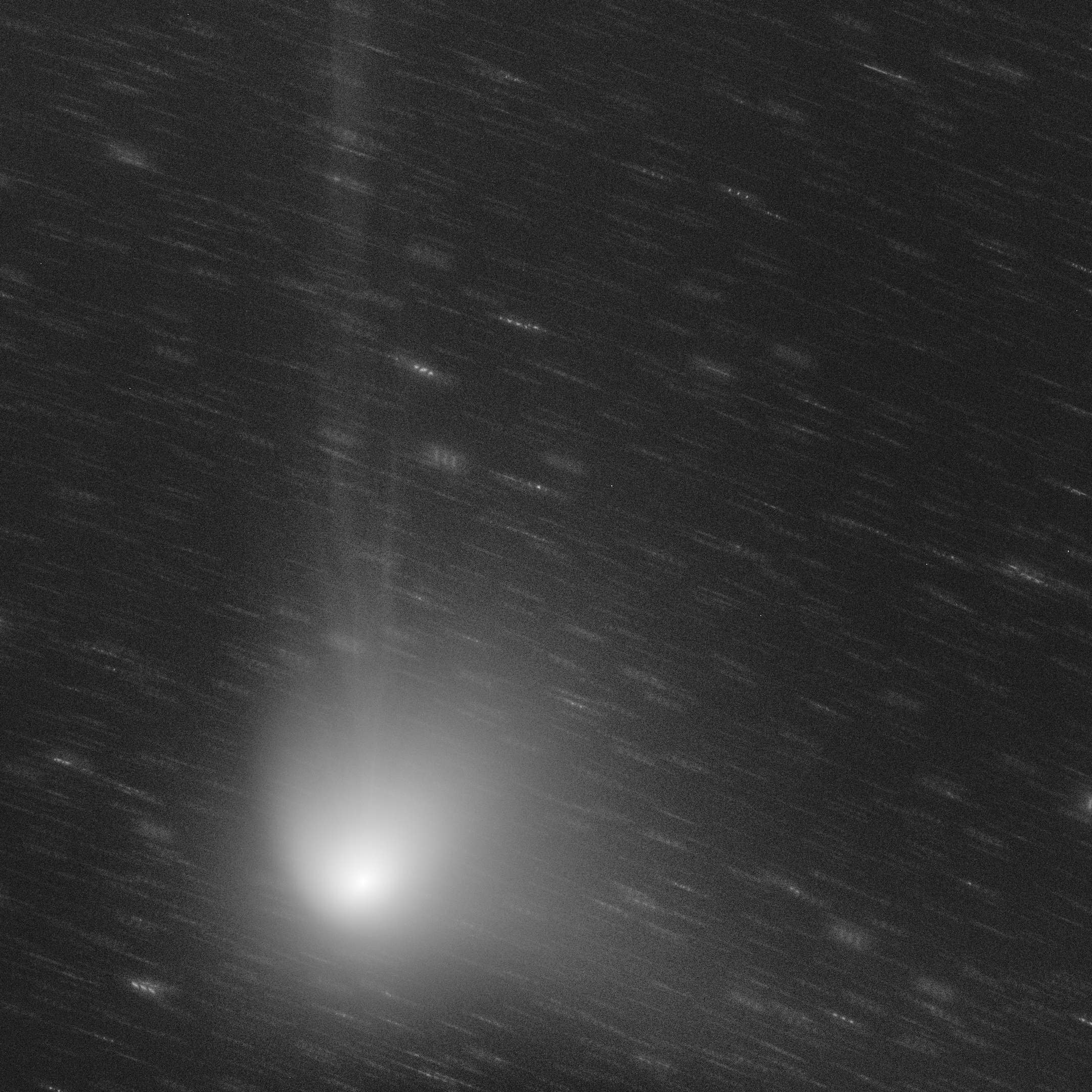
To bring the comet to the foreground, we decided to apply a median combination because it diminishes the brightness of the trailing stars without the need to use a pixel rejection. The result on a single frame can be seen below:

Our intention when imaging comets has never been to show them over a still star field since they are, in fact, moving objects. So the present work of art is focused on showing exactly what it is: a beautiful comet moving over a star field.

We created the videos with DaVinci Resolve, but you can make them in PixInsight as well by using the Blink tool. First, you'll need to install FFmpeg on your computer. Once installed, Blink will use it to create the movie. In Blink, you need to click the clapperboard button to access the video creation menu:

Once in the video creation menu, we recommend using the following arguments for FFmpeg:

-r 25 -vf yadif,format=yuv420p -force_key_frames "expr:gte(t,n_forced*2)" -c:v libx264 -b:v 45M -bf 2 -c:a flac -ac 2 -ar 44100 -strict -2 -use_editlist 0 -movflags +faststart output.mp4

This encodes the video to a format fully compatible with YouTube and mobile devices. You only need to take into account two arguments:

• The frame rate is defined by the "-r" argument. Set it at the speed you want in frames per second.
• You can control the compression level by changing the video bitrate specified by the "-b:v" argument. In the case above it's 45 Mb. Lower values will generate smaller and more compressed videos.
• You can change the filename of the generated video by changing "output.mp4" to the desired name.

Applying SPCC to Comet Images

If we want to apply PCC or SPCC to calibrate the color of this comet, we'll have a problem: these tools calculate the RGB factors based on stellar photometry, but in our RGB images we only have star trails. We describe in this section what we did to overcome this problem, which was a mix of observational and processing workflows.

On the observational side, we started observing the comet with a short sequence of RGB exposures: 6x15 seconds in each filter. Although the telescope was tracking the comet in these exposures, the stars were almost round. We used these images to reference the color of the long-exposure picture.

After this short sequence, we start the main imaging sequence, composed of 2-minute exposures on RGB filters. We preprocess everything in WBPP but only use it to calibrate the images. Here is the Lights tab in the script:

Now we'll generate three sets of masters:

• First, we run CometAlignment with both the short and long-exposure images. This is done in a single run because, in this way, both image sets will have the comet in the same position. Then, we integrate the masters of comet-aligned images separately. So, in the end, we have six masters: the 15-second R, G and B, and the 2-minute R, G and B. From these masters we compose the 15-second and 2-minute RGB images with ChannelCombination.
• We now run StarAlignment on the 15-second exposures that came out directly from WBPP without aligning to the comet. This will align the stars. Then, we integrate the three small sets and combine an RGB image in ChannelCombination. As a result, we now have a third master, which is a color image with the stars aligned and the comet misaligned.

Below you can see a mouseover comparison of the three master color images:

The critical part of this workflow is in how we integrate the short-exposure masters, because what we want to do is to translate the color balancing from the image aligned to the stars to the one aligned to the comet. Since these short exposures were acquired during a short period, we'll apply an ImageIntegration process without any scaling or weighting.:

This ensures that both color images are exactly the same in terms of signal intensity. Now, we can calculate the correct color balance in the picture with the stars aligned. We set the white point to a G2V star (a Sun-like star) because the comet's dust tail and head reflect the sunlight.:

Once we execute SPCC on it, we will get the RGB factors from the console:

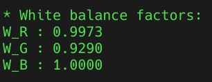
These factors are the key to correcting the color of the long-exposure image. First, we'll transfer this color balance to the short-exposure master aligned to the comet. We'll perform this with ColorCalibration by applying a manual white balance. We uncheck the structure detection and check the manual white balance section, where we'll write the RGB factors previously calculated with SPCC. The complete tool configuration can be seen below:

We applied this process to the 15-second RGB master aligned to the comet. This way, we transferred the color calibration from the star-aligned to the comet-aligned image. Please remember that ColorCalibration does not apply any background neutralization. At this point, don't worry if the sky background has a strong color cast because we'll correct it at the end of the workflow on the long-exposure image

Once the 15-second comet-aligned master has the right RGB balance, we need to transfer this color calibration to the long-exposure image. This can be done with LinearFit. Ideally, we could set the short-exposure image as a reference for LinearFit. But, in the real world, this will never work well because most of the image is pure background, and the comet covers only a small part of the field of view. To calculate a robust fit, we create two small previews over the comet heads and create new images from them (please watch our videos about view actions on the official PixInsight YouTube channel). We'll calculate the linear fit over these areas with significative signal from the comet.

In LinearFit, we set the 15-second image preview as the reference and apply it to the 2-minute image preview. Then, the tool outputs the fitting equations to the console. The RGB factors we need to know are pointed out below:

With these numbers we can apply again ColorCalibration to the long-exposure image with a manual white balance:

After this process, we finally perform a background neutralization process on the long-exposure image to finish the color correction workflow: