1 Introduction
[hide]
When we measure color using photometric techniques, the camera integrates all the light that each filter transmits. For each measured star, this sum gives us the star's brightness in that filter, so we reduce all transmitted light to a single number. Then, by comparing it to the brightness in another filter, we get the star's color index.
This is a source of errors. Suppose we have a very red star. Suppose also that our camera is quite insensitive to the extreme range of red light. This will cause the star to appear dimmer in the red filter, despite using the same filters as other observers who own a more red–sensitive camera, which will undoubtedly affect our color measurements.
The same happens when we relate the colors observed through the photometric filters used by a photometric catalog, such as APASS,[1], with the colors observed through our RGB filters. As the two systems have entirely different transmission curves, this simplified color conversion has an implicit uncertainty. To this conversion effect, we should also add the implicit uncertainty in the photometric measurements of the APASS catalog. All these factors lead to a color calibration limited by this color conversion and not by the noise in the image.
So far, we have been basing photometric color calibration on the APASS catalog in PixInsight. APASS was the first stellar catalog fulfilling the requirements for this task by providing measurements made with CCD cameras and filters similar to the photographic RGB filters that we normally use for a significant amount of stars (about 120 million stars in APASS Data Release 10). The availability of APASS led to the development of our PhotometricColorCalibration tool (PCC). With PixInsight's new generation of photometric and color calibration tools, we now take a step forward by basing all measurements on data from the Gaia space mission.[2] [3]
Gaia currently represents the state of the art in terms of stellar astrometry and photometry. The star catalogs and auxiliary data generated by Gaia are of the highest quality as they are based on measurements made from space. We at the PixInsight Development Team have already been using and recommending Gaia for all astrometry–related tasks in PixInsight for many years. Now we have implemented a new tool, SpectrophotometricColorCalibration (SPCC), which uses Gaia's mean BP/RP spectra[4] available since Gaia Data Release 3.[5] [6] [7] SPCC is the first of a series of tools we are developing to exploit the availability of Gaia mean spectrum data in PixInsight.
Spectrophotometry consists of applying photometry separately to individual wavelengths. We can achieve this using a spectroscope or a system of juxtaposed narrow filters. With Gaia spectrophotometry, instead of having a few isolated brightness values, we now have a continuous spectrum function for each star, which we can sample arbitrarily from ultraviolet to infrared.
The great advantage of spectrophotometry is that it allows us to compute the brightness that a star should have through the exact filters we have used to acquire our image. This is done by simply multiplying each filter's transmission curve by the star's spectrum. In addition, we can also synthesize the exact colors that a white reference should have as acquired with our filters. By taking into account the spectra and the transmission curves, we get rid of the important sources of errors mentioned above—when comparing PCC fitting graphs with the corresponding SPCC graphs, in most cases, the uncertainty of computed white balance functions is decreased by more than one order of magnitude.
Gaia provides the first accurate, massive spectrophotometric catalog in the history of astronomy. Compared to APASS, Gaia offers unprecedented uniform sky coverage and color homogeneity since the data are based on observations made from space without the varying conditions of the atmosphere. We now have at our fingertips the spectra of about 219 million stars, which, considering that each spectrum is made up of more than 300 measurements, represents a base of 80 billion data. This database is now available for download to all PixInsight users from the PixInsight Software Distribution System as a set of XPSD database files, ready to be used with the new SPCC tool. SPCC, therefore, represents a significant step forward in terms of robustness and reliability, and a new milestone in the definition and expression of color in astrophotography.
2 The White Reference
[hide]
Philosophical criteria must always support the definition of a standardized white reference. The definitions of many of the measurement units of the International System of Units follow this reasoning, so we could say that this is a work in the philosophy of science and mathematics field. For example, the definition of the degree Celsius and that of the liter in its origin, are related to one of the essential elements for life: water.
Contrarily to many other imaging disciplines, in the case of astrophotography, the problem of color is not primarily a matter of accuracy. In astrophotography, what we need to be precise about is the concept that supports color in our images. When we designed PCC, we established a new color philosophy based on a reference point more universal than sunlight: an average spiral galaxy.[8] [9] The reasoning behind this conceptual change is based on two principles:
- The Sun does not illuminate the deep sky astronomical scene.
- A spiral galaxy works as a balance point because, as a whole, it has a significant representation of all stellar populations.
At that time, we decided that this reference spiral galaxy would have an average spectrum between the Sb, Sc and Sd types, avoiding the extreme types and leaving out the lenticular (S0) galaxies. Since the release of the SPCC and PCC tools in November of 2022, we have updated this definition of an average spiral galaxy to be the mean of the spectra of all morphological types: S0, Sa, Sb, Sc, Sd, and Sdm.
The rationale of this decision is that, in this way, we are fairer when averaging the different stellar populations, especially those of galaxies with a high rate of star formation (Sd and Sdm), as we can see in Figure [1].

While the morphological types S0, Sa, Sb and Sc have similar spectra, the types Sd and Sdm have much more emission in the blue part of the visible spectrum. By averaging all of these spectra, the spectrum of the average spiral galaxy (plotted with a dashed line) is very similar to that of a type Sc galaxy, as shown in the graph above. A very representative galaxy of this morphological type is M74 (Figure [2]).
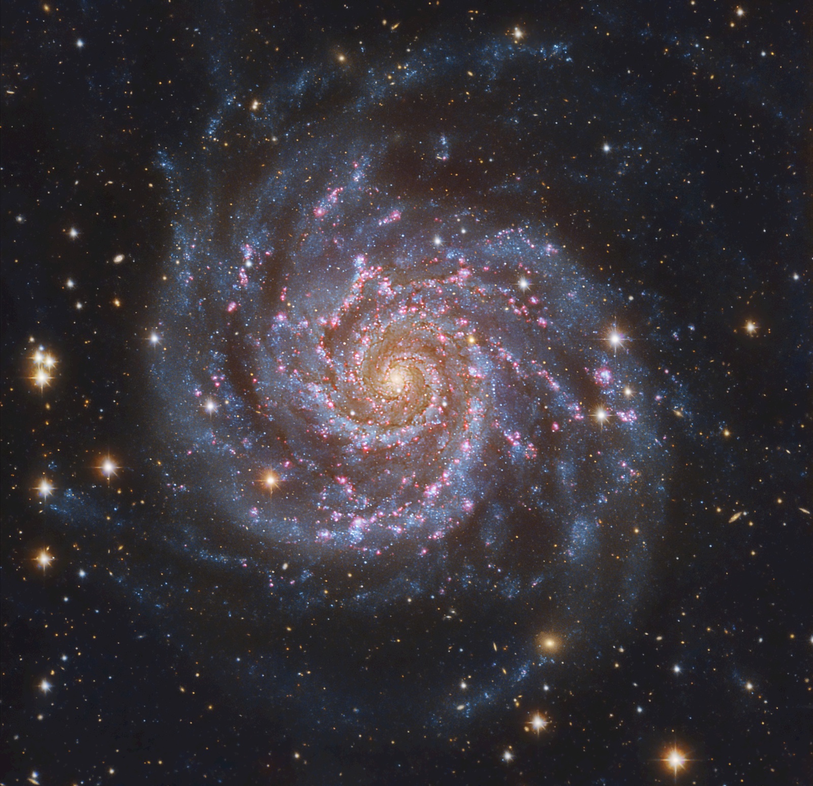
Figure 2 — Messier 74, a face–on Sc galaxy representative of our average spiral galaxy white reference.
Image credits: CAHA, Descubre Foundation, DSA, OAUV, Vicent Peris (OAUV/PixInsight), José Luis Lamadrid (CEFCA), Jack Harvey (SSRO), Steve Mazlin (SSRO), Oriol Lehmkhul, Ivette Rodríguez, Juan Conejero (PixInsight).
The formal definition of our average spiral galaxy white reference is then as follows:
Therefore, this is the new standard white reference on which color calibration will be based in PixInsight, both photometric color calibration with PCC and spectrophotometric color calibration with SPCC.
3 Gaia Mean BP/RP Spectrum Databases
[hide]
With the release of version 1.8.8-6 of PixInsight in October 2020, we introduced XPSD (eXtensible Point Source Database), a new database format we have designed and developed for fast and efficient access to massive astrometric and photometric star catalogs. As of writing this document, we have already released XPSD databases with data from the APASS DR9, APASS DR10, Gaia DR2, Gaia EDR3, and Gaia DR3 catalogs.
Before XPSD, our astrometry and photometry tools and scripts relied on online database access services, such as VizieR.[12] These online services are excellent in their implementation and capabilities. They have made possible the development of robust, accurate, and feature–rich software products such as our well–known ImageSolver, AperturePhotometry and AnnotateImage scripts, among others. However, for the requirements of most of these tools and many others subject to intense development work in PixInsight, we need much faster access to huge astronomical catalogs. The main advantage of the XPSD format is that it provides efficient access to massive astronomical catalogs using local database files, that is, files stored on the local filesystems of the user's machines or local networks.
The XPSD format is similar to the XISF image format[13] in the way it stores and organizes metadata—for example, both formats use XML file headers to guarantee flexibility and extensibility in metadata serialization. XPSD files provide fast, multithreaded access to point source data with special quadtree–based index structures to perform search operations on arbitrary regions of the celestial sphere, as well as efficient storage with transparent data decompression. An in–depth, formal description of the XPSD format is beyond the scope of this document, so we'll limit the following subsections to describe the practical usage of XPSD databases with the SPCC process. For interested developers, the implementation of XPSD and currently supported catalogs in XPSD format (APASS and Gaia as of writing this document) is part of our open–source C++ development framework.[14]
3.1 Using the Gaia Process with SPCC

XPSD database support follows a client–server design in current versions of PixInsight. The Gaia process provides access to local Gaia DR2, EDR3 and DR3 databases working as a server for scripts and modules, allowing them to perform arbitrary, thread–safe search operations on Gaia catalogs. The Gaia process can also be used as a standalone tool thanks to its graphical user interface, which you can see above, but describing this functionality is out of the scope of this document.
Before using Gaia with SPCC, you have to install a set of database files, as we'll describe now.
3.1.1 Configuring Gaia DR3/SP Database Files for SPCC
The new SPCC process requires special Gaia DR3/SP databases. DR3/SP means here Data Release 3 with spectra. These XPSD databases provide astrometric, photometric and sampled mean BP/RP spectrum data for a total of 219,165,266 Gaia DR3 point sources. Available data include equatorial coordinates, proper motions, parallax, mean G, BP and RP magnitudes, and mean spectra from 336 to 1020 nm sampled discretely at 2 nm steps (343 spectrum values) for each star.
Gaia XPSD database files can be downloaded from our Software Distribution interface, available to all PixInsight licensed users on our corporate website at the following URL:
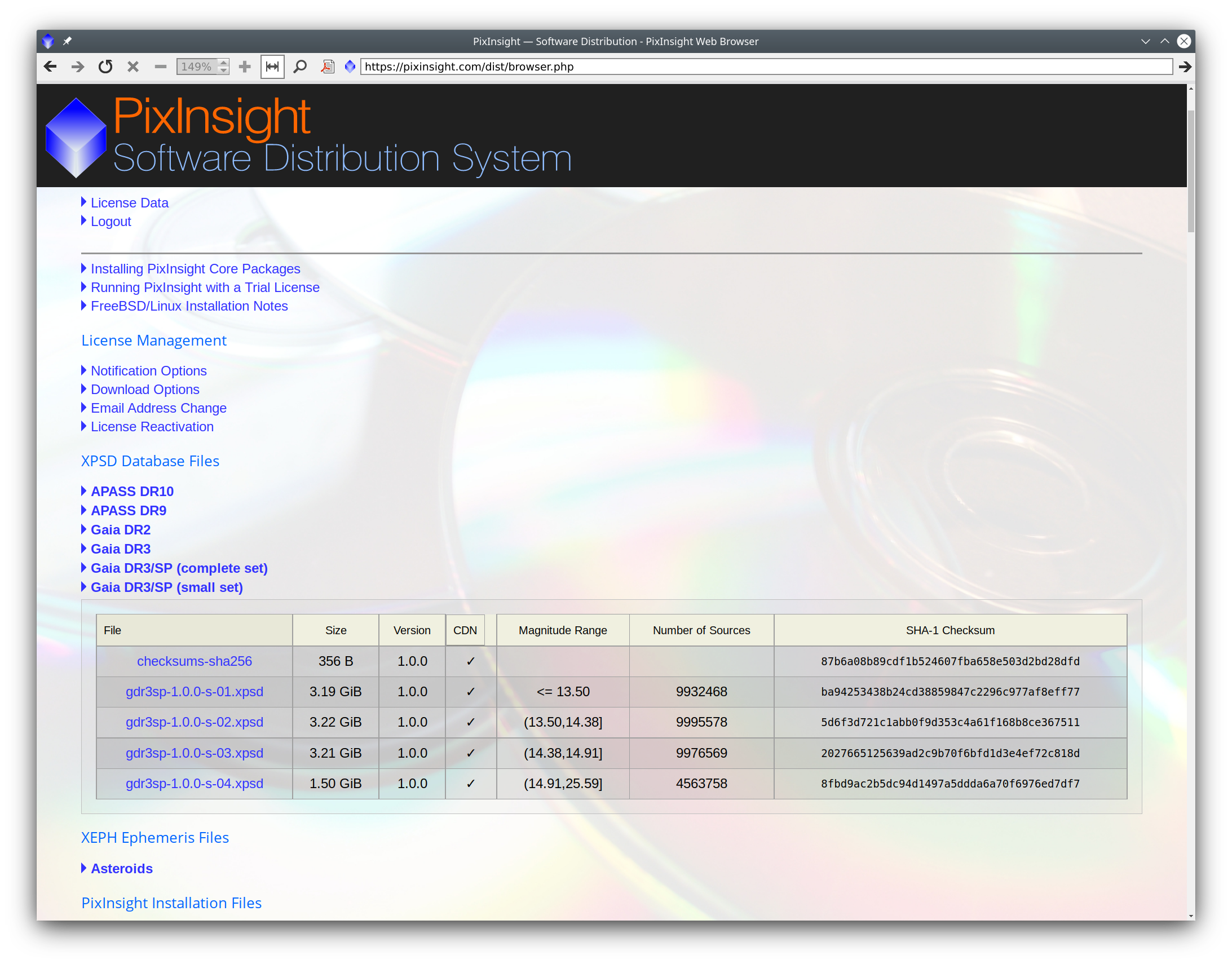
Currently we provide two sets of Gaia DR3/SP database files:
- The small set, which includes 4 database files with 34,468,373 stars. This set requires 11.1 GiB of disk storage space. This set is normally sufficient for calibrating wide to moderate field images.
- The complete set, with 20 database files and the full set of 219,165,266 stars. This set requires 63.2 GiB of disk storage space. The complete set can be necessary for the calibration of narrow field images, plus it provides the possibility to increase the number of spectra used for enhanced color calibration accuracy. If disk space availability is not a problem, this is the recommended option.
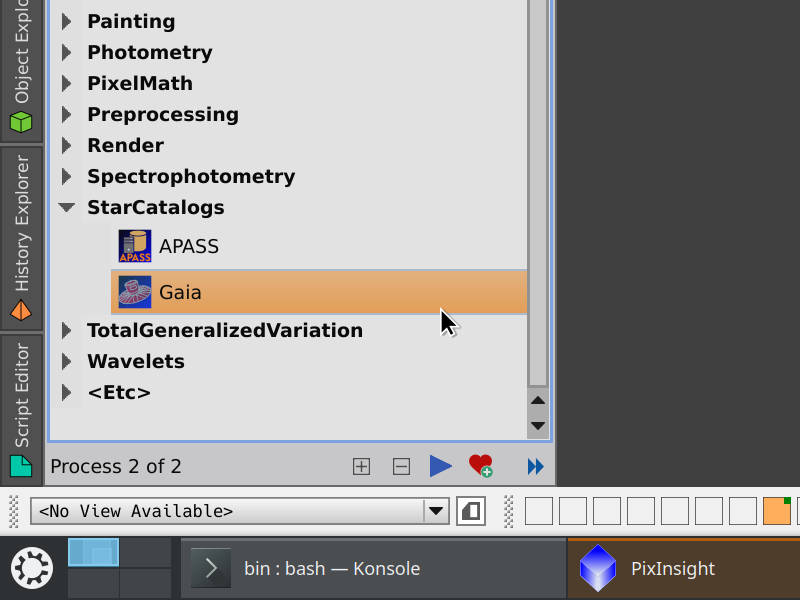
Before using the SPCC process, you must configure the Gaia process to use Gaia DR3/SP local database files. First, download the required .xpsd files, either the small or complete set, at your option. Then open the Gaia process from the Process Explorer window, where you'll find it under the StarCatalogs and Astrometry categories:
On the Gaia process window, click the Preferences button (with a wrench icon) to open the Gaia Preferences dialog:
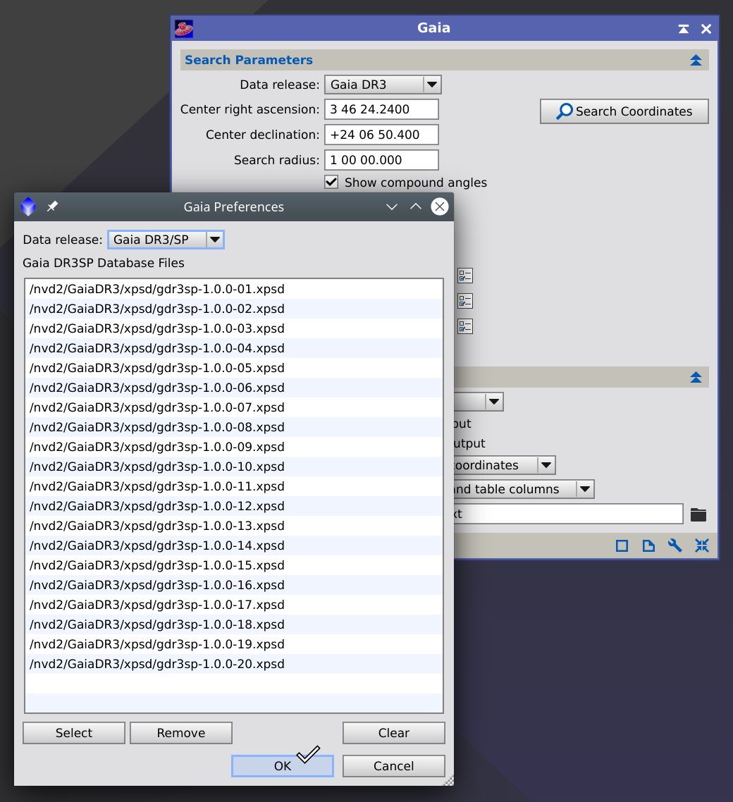
On Gaia Preferences, select the Gaia DR3/SP data release, click the Select button to select the required .xpsd files, and click the OK button. Now you can use the SPCC process with full access to local XPSD database files.
Warning — Never mix .xpsd files from the small and complete Gaia DR3/SP sets. Doing so may lead to incorrect color calibration results due to duplicate database entries.
4 Spectrophotometry–Based Color Calibration Algorithm
[hide]
This section describes the algorithms we have designed and implemented for the new SpectrophotometricColorCalibration process (SPCC) in PixInsight. At a high level, we can decompose the SPCC task into the following main steps:
- Star detection. Detect sources separately on each color component of the image.
- PSF fitting. A point spread function (PSF) is fitted for each detected source, also separately for individual RGB channels.
- Signal evaluation. For each detected source, compute three flux estimates, respectively for the R, G and B color components. Evaluate pixel values within the fitted elliptical PSF region (at the one-tenth maximum level (FWTM) by default).
- Database search. Perform a database search to retrieve the set of Gaia DR3 stars with mean spectra within the region of the sky covered by the image. This requires the image to provide a valid astrometric solution.
- Source matching. Find the set of pair matches between Gaia DR3 catalog stars and detected stars on the image.
- Image flux ratios. For each matched image star, compute its R/G and B/G image flux ratios from the corresponding PSF flux estimates.
- Catalog flux ratios. For each matched catalog star, integrate its spectrum multiplied by each color filter and an optional quantum efficiency (QE) curve. Compute the R/G and B/G catalog flux ratios from the values of these integrals.
- White reference ratios. For the selected white reference, integrate its spectrum multiplied by each color filter and an optional quantum efficiency (QE) curve. Compute the R/G and B/G white reference ratios from the values of these integrals.
- White balance functions. Compute robust linear fits from the set of matched catalog and image R/G and B/G flux ratios.
- White balance factors. Use the white reference ratios as input to the white balance functions to find the R, G and B white balance factors. These factors are applied by multiplication with the color components of the image to perform a white balance operation.
- Background Neutralization (optional). Subtract any existing bias in the color components after the white balance operation, measured on a subset of pixel samples representative of the sky background as acquired in the image.
We describe these steps in the following subsections, including some important implementation details.
4.1 Star Detection / PSF Fitting
We begin by detecting a set of point sources in the image. This first step is critical because we want to detect stars, not extended objects or potential bright artifacts such as uncorrected hot pixels, cosmic ray impacts, satellite and plane trail residuals, etc. We already have this task well implemented in our code base and have been improving it for many years.
The second step is fitting a point spread function (PSF) to each detected star. Our implementation of PSF fitting is based on the Levenberg–Marquardt[15] algorithm and has also been part of our code base for a long time. We have substantially improved these fitting routines in recent versions of PixInsight. Our current implementation supports elliptical Gaussian and Moffat[16] functions for PSF flux evaluation. These functions are given by
 [1]
[1]and
 [2]
[2]respectively, where the parameters are:
-

-
Average local background.
-

-
Amplitude, which is the maximum value of the fitted PSF, and also the function's value at the centroid coordinates.
-

-
Centroid coordinates in pixel units. This is the position of the center of symmetry of the fitted PSF.
-

-
Standard deviations of the PSF distribution on the horizontal and vertical axes, measured in pixels. Conventionally, the X axis corresponds to the direction of the semi–major axis of the fitted elliptical function.
-

-
Moffat shape parameter.

Figure 3 — Some point spread function profiles. The full width at half maximum (FWHM) and full width at tenth maximum (FWTM) are standard measures to quantify the dimensions of a fitted PSF.
4.1.1 Rotated Functions
When the difference between  and
and  is larger than the nominal fitting resolution (0.01 pixel in the current implementation), our PSF fitting routines fit an additional
  parameter, which is the rotation angle of the X axis with respect to the centroid position. varies in the range [0°,180°). For a rotated PSF, the
  and
and  coordinates in the above equations must be replaced by their rotated counterparts
  and
and  respectively:
 [3]
[3]4.1.2 Adaptive Sampling Region
Each PSF is fitted from pixels inside a square sampling region centered at the approximate central coordinates of the detected source. The size of each sampling region is determined adaptively by a median stabilization algorithm. The sampling region starts at the limits of the detected source structure and grows iteratively until no significant change can be detected in the median calculated from all pixels within the region. This technique improves accuracy and resilience to outliers in fitted local background estimates, which are crucial for the accuracy of fitted PSF models and hence of PSF flux estimates.

4.1.3 Automatic PSF Type Selection
Our current implementation supports an automatic mode for selecting an optimal PSF type for each detected source. When this mode is enabled, a series of different PSFs will be fitted for each source, and the fit that leads to the least absolute difference among function values and sampled pixel values will be used for flux measurement. Currently, the following functions are tested in this special automatic mode: Moffat functions with shape parameters equal to 2.5, 4, 6 and 10 (Figure [5]). This limited set represents a compromise between accuracy and efficiency with current computational resources. In future versions, we'll add more sophistication to this adaptive PSF type selection strategy.

4.2 PSF Flux Evaluation
Once we have a set of  detected sources with their corresponding fitted point spread functions for each color component
  , we compute three PSF flux estimates for each source:
 [4]
[4]where  is the elliptical detection region, defined by default at the one tenth maximum level (FWTM) of the fitted PSF,
  represents a set of image coordinates within
  ,
,  is the pixel sample value at , and
  is the fitted local background estimate.
Note that fitted (amplitude) parameters are not used for PSF flux evaluation, since flux is calculated exclusively from sampled image pixels. This leads to our hybrid PSF/aperture photometry approach.
4.3 Database Search / Star Matching
Once we have gathered flux estimates for each detected and fitted star in the image's red, green and blue channels, we need to find a corresponding set of sources with mean BP/RP spectra in the Gaia DR3 catalog. For this task, the image must provide a valid astrometric solution, which can be computed with our standard ImageSolver script. We strongly recommend our astrometric solutions based on thin plate splines[17] instead of standard WCS linear solutions. Our spline–based solutions provide accurate local distortion corrections that are impossible with standard linear or polynomial WCS solutions.
Our XPSD Gaia DR3/SP database provides fast access to the entire set of 219,165,266 Gaia DR3/SP stars with positional, photometric and spectrum data: equatorial coordinates, proper motions, parallaxes, mean BP, G and RP magnitudes, and sampled spectra from 336 to 1020 nm. We perform a database search operation to find Gaia DR3/SP stars within the region of the sky covered by the image. We limit this search to a G magnitude limit appropriate for the field of view of the image, which we find iteratively by performing auxiliary database search operations following a binary search scheme. These operations typically require less than one second with relatively fast, consumer–grade SSD devices.
Once we have image coordinates for all catalog stars, we generate a bucket point–region quadtree structure[18] [19] to match pairs of stars with the help of fast spatial indexed access.
4.3.1 Reduction of Positions
The catalog sources are mapped to sources detected on the image by transforming their equatorial coordinates to Cartesian coordinates on the image plane. For this transformation, we first apply the appropriate reduction of positions,[20] [21] which depends on the celestial reference system to which the astrometric solution has been referred:
- ICRS: astrometric positions. This applies space motion corrections accumulated since the epoch of catalog coordinates (2016.0 for Gaia DR3), including parallax and proper motions, with corrections for the relativistic Doppler effect, as well as the effect of relativistic deflection of light due to solar gravitation.
- GCRS: proper positions. This includes the same corrections computed for astrometric positions, plus the effect of the aberration of light, including relativistic terms.
- Geocentric apparent system: apparent positions. This includes the same corrections computed for proper positions, plus frame bias, precession and nutation. The origin of right ascensions is the true equinox of date.
When image metadata includes the geodetic coordinates of the observation location (longitude, latitude and height), topocentric places are calculated as appropriate.
4.4 Image and Catalog Flux Ratios
At this point we have matched image/catalog pairs of stars. For each matched image star, we compute the following image flux ratios:
 [5]
[5]Now let's define the following functions:
-

-
The filter functions, respectively for the red, green and blue color components. These are three continuous functions of wavelength, where the dependent variable is filter transmission in the [0,1] range. These functions should describe the spectral response of the filters used to acquire raw image data.
-

-
The spectrum of a matched star,
 , which has been retrieved from the Gaia DR3 catalog. This is a continuous function of wavelength whose value is expressed in spectral photon flux units:
  .
. -

-
A quantum efficiency (QE) curve. This is also a continuous function of wavelength with values in the [0,1] range. This function is optional; by default, it is an ideal QE curve with a constant value equal to 1. Under normal working conditions, a QE curve is only necessary for monochrome sensors. For color sensors and cameras, one assumes that quantum efficiency is being taken into account implicitly by the corresponding filter spectral response curves.
All these functions are evaluated from sampled data with our implementation of Akima subspline interpolation.[22] [23]
The catalog color samples are given by
 [6]
[6]where the integration interval  is determined by the availability of filter, spectrum and efficiency curve data retrieved from working databases. With our current XPSD database implementation, sampled Gaia DR3 spectra are available from 336 nm to 1020 nm, so this is the widest possible practical range of wavelengths that can be applied. Filter and QE curve ranges vary largely among different filters, sensors and cameras.
We evaluate the above functions by numerical integration, with a default step size of 0.1 nm, applying a simple Simpson's 1/3 rule.[24]
The catalog flux ratios are now defined as
 [7]
[7]4.5 White Reference Ratios
Let  be the selected white reference spectrum, which is a continuous function of wavelength with values expressed in spectral photon flux units. As the rest of curve functions described in the preceding section, this function is also interpolated [22] [23] from sampled spectra. The white reference samples are
 [8]
[8]As before, these equations are evaluated by numerical integration.[24] The white reference ratios are then given by
 [9]
[9]4.6 Robust Linear Regression
From the sets of matched catalog and image stars, we define the following point vectors:
 [10]
[10]Each component of these vectors is a pair of matched catalog/image flux ratios. Taking catalog flux ratio as the explanatory variable and image flux ratio as the dependent variable, we fit the following linear functions, respectively for  and
and  :
:
 [11]
[11]The sets of image flux ratios often contain significant fractions of outliers, i.e., values that depart significantly from the expected linear trend in these functional fits. These differences can be due to a variety of factors, including deficient filter characterization, deficient quantum efficiency curve characterization, image noise, nonlinearity of image data, and the fact that we are neglecting the effect of atmospheric dispersion in this initial version of the SPCC process.
We have implemented a linear fitting routine based on the repeated median regression algorithm[25] [26] for slope evaluation. Repeated median regression is a robust linear regression algorithm with a finite sample breakdown point[27] of 0.5, which means that it can tolerate up to a 50% of outliers in the input point vectors, including arbitrarily large or small values, without degradation of the fitted function. These linear fits represent a crucial step in the color calibration algorithm, where accuracy and robustness are of extreme importance to the quality of the final calibrated result.

Figure 6 — Some well–known linear regression methods compared to our implementation of the repeated median robust regression algorithm. In this example, we have applied each algorithm for SPCC color calibration under significant outlier contamination. Our implementation can detect the true linear trend in the cloud of data points, while other non–robust methods are clearly influenced by a large number of outliers at the upper side of the graph.
4.7 White Balance Factors
The white balance factors are given by
 [12]
[12]which we normalize to form a unit vector:
 [13]
[13]These normalized factors are applied by pixel–wise multiplication to the image's red, green and blue channels, respectively, to perform the white balance correction.
4.8 Robust Background Neutralization
After the white balance correction, an optional background neutralization removes any existing bias in the image to achieve neutral average pixel sample values for a specified background reference. The background reference should generally be a subset of pixels representative of the sky background as acquired in the image being calibrated, although neither the algorithm specification nor the current implementation imposes any restriction in this regard.
Let  be the background reference region in image coordinates, and let
  be the set of pixel sample values for a color component and for all image pixel coordinates within . Define:
 [14]
[14]where  is the median absolute deviation from the median, and the scale factor 1.4826 makes it consistent with the standard deviation of a normal distribution. Let
  and
and  be, respectively, the lower and upper limits of the background sampling range, expressed in sigma units. Then the background sampling range bounds are given by
 [15]
[15]In the current implementation, the default background sampling limits are
 [16]
[16]These limits are user–selectable, although their default values usually work well in most cases. Note that we are introducing adaptability in the background neutralization algorithm by defining these limits in sigma units instead of literal pixel values.
Now, if is a pixel sample value at image coordinates for a color component , the corresponding background reference value is
 [17]
[17]The background neutralization operation is a pixel–wise subtraction of each  from its respective color component.
5 Spectrophotometric vs Photometric Color Calibration
[hide]
The main advantage of Gaia over APASS is its greater accuracy and consistency throughout the entire sky. You can easily find images where uncertainty in the APASS catalog is locally quite high, leading to results where the precision of color calibration is quite low. In these cases, color precision is not limited by image noise but by noise in the colors derived from catalog data. Let's see an example with the following wide–field image of NGC 6946.
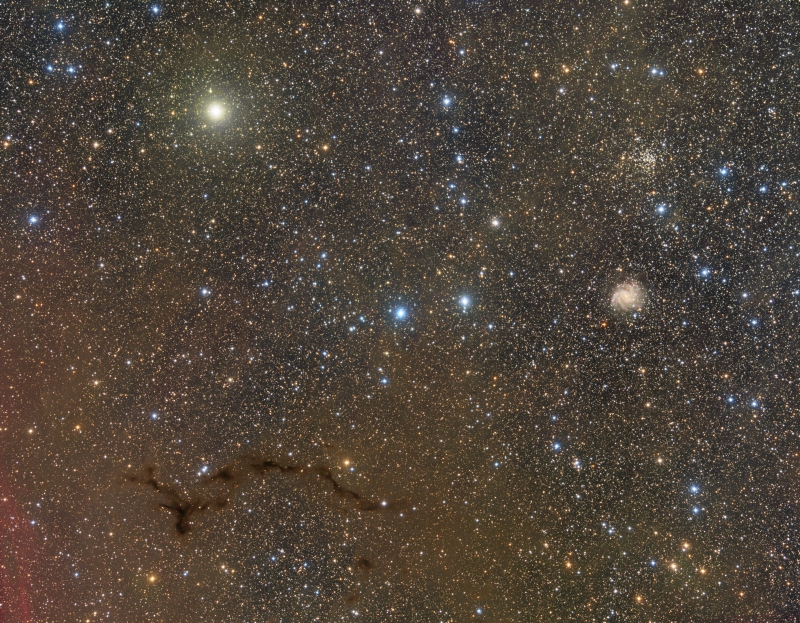
We will compare the uncertainties in the R scaling factor calculated with the APASS and Gaia catalogs. When we increase the limiting magnitude, we expect to get an increase in uncertainty because the fainter stars are noisier in our image. On the contrary, when we limit calibration to brighter stars, we expect to see a decrease in uncertainty. This is exactly what happens when we vary the limiting magnitude from 14 to 17 using the Gaia catalog (Figure [7]).
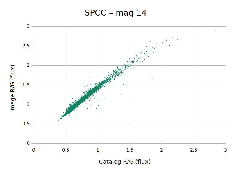
Figure 7 — Catalog and image flux ratios for the red channel of the NGC 6946 test image as a function of limit magnitude, using Gaia DR3 mean BP/RP spectra.
As we would expect, limiting catalog stars to 14 magnitude leaves a very well–defined line because we are using stars with a higher signal–to–noise ratio in the image. This is not the case with APASS in this field, as can be seen in Figure [8].
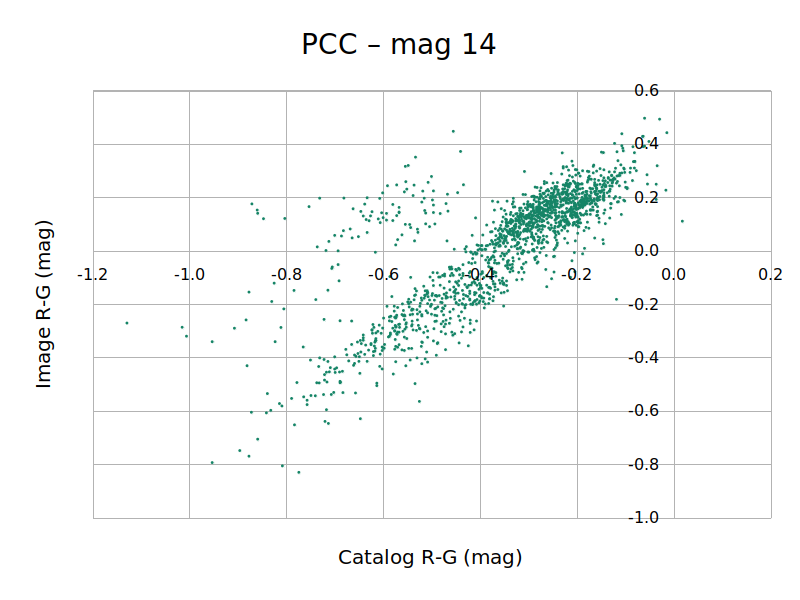
Figure 8 — Catalog and image flux ratios for the red channel of the NGC 6946 test image as a function of limit magnitude, using APASS DR10 photometric data.
In Figure [8] we observe that the point cloud does not tend to a thin distribution when we limit the catalog magnitude to 14. In other words, we cannot decrease uncertainty by decreasing the limiting magnitude from 15 to 14. Moreover, if you look carefully at the graphs, you will notice that increasing the limiting magnitude increases the dispersion of the points, mainly in the horizontal direction. This means one thing: APASS data are noisier than our image, so color calibration is limited by the precision of APASS and not by the image itself. Note also that, in the graphs of Figure [8], there are clusters of stars that fall entirely out of the main trend, denoting local biases in the APASS catalog.
The Gaia catalog outperforms APASS in all of these aspects. We routinely get much smaller color calibration uncertainties by using Gaia spectrum data. We have compared the R and B scaling uncertainties in a test performed with 21 broadband deep sky images. The graph in Figure [9] shows the decrease in uncertainty achieved using SPCC instead of PCC.

Figure 9 — Uncertainty reduction achieved in color calibrations performed with the SPCC tool (Gaia DR3 mean BP/RP spectra) with respect to calibrations performed with PCC (APASS DR10 photometric data). Uncertainty is being evaluated as the dispersion of line slopes evaluated during robust linear regression.
Almost in every case, we find a substantial increase in the precision of color calibration. In some cases, the color adjustment is about ten times less uncertain. On average, we expect a reduction of color calibration uncertainties by 400% and 300%, respectively for the red and blue channels.
Overall, we have found that color calibrations performed using Gaia spectra (SPCC) lead to calibrated images with a slight blue shift compared to calibrations using APASS photometry (PCC). Usually, this blue shift is under 10%. To verify this, we first performed a calibration with PCC and then calibrated again with SPCC. Ideally, SPCC would find 1:1:1 RGB white balance factors, but the calculated ones are systematically lowering the R and G components. This is shown in Figure [10].
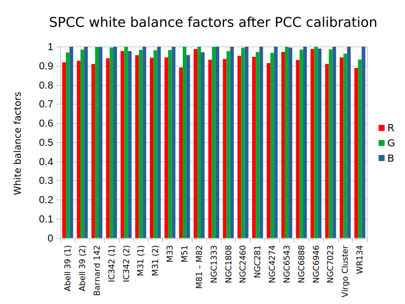
Figure 10 — White balance factors calculated by the SPCC tool (Gaia DR3 mean BP/RP spectra) for images previously calibrated with the PCC tool (APASS DR10 photometric data).
The differences in white balance factors and calibration uncertainty between both catalogs are not consistent throughout this set of test images. However, since the precision in color measurements is so higher with Gaia, we are much more confident with this catalog not showing any global or local color shifts, as well as on the vastly superior accuracy of color calibrations performed using Gaia. Gaia mean BP/RP spectra represent the current state of the art for flux measurement and will be the present and future source for photometry calculations in PixInsight.
6 The SpectrophotometricColorCalibration Tool
[hide]
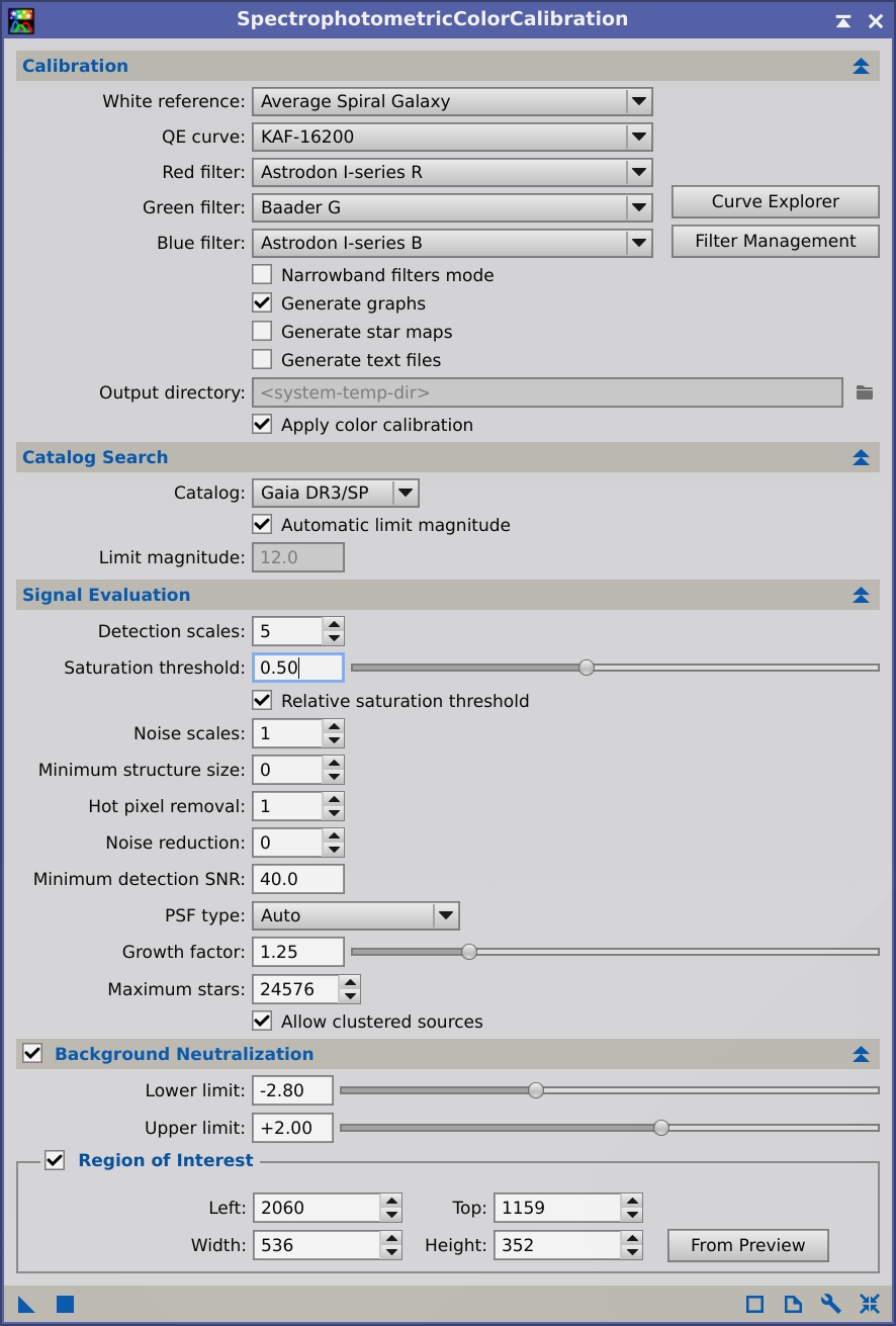
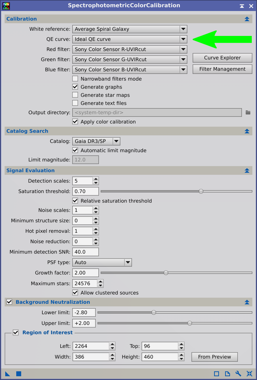
The user interface of SpectrophotometricColorCalibration (SPCC) is quite similar to the interface of PhotometricColorCalibration (PCC):

Switching from PCC to SPCC is straightforward. In both tools, we have the Catalog Search, Signal Evaluation and Background Neutralization sections. The only significant difference between these tools, for basic usage, is the ability to configure our own filters provided by SPCC. In PCC, we compare stars measured on our RGB image channels to the brightness of the same stars measured with the photometric filters used to build the APASS catalog. With the Gaia spectra database, we calculate the exact brightness of each star in the filters we have used to acquire our image. Hence, in the Calibration section, we can assign a filter for each color channel of the image:

Irrespective of being a color image acquired with a monochrome or color camera, we should always select the three filters separately. As shown above, the default filters are those of a generic Sony color image sensor. The only difference regarding the type of camera is that, for a monochrome camera, we first need to create a color image with the ChannelCombination tool, as explained in the next section.
In the default filter list, we have included the most common filter sets:
- Astrodon E and I series.
- Astronomik.
- Baader.
- Chroma.
- Selected models of Canon, Nikon and Pentax DSLRs.
- A generic Sony color image sensor with three options (sensitivity from UV to IR, with UV-cut filter and with UV and IR-cut filter).
- Astronomical standard photometric filter sets: Johnson UBVRI and Sloan u'g'r'i'z'.
As you can see, most filter sets are split in the three drop–down lists. This is because most of the filters can be assigned only to one primary color. For example, there is no sense in assigning the Baader G filter to the R channel, so the Baader G filter only appears in the Green filter drop–down list. This limitation does not exist for photometric Johnson and Sloan filters since their passbands range from ultraviolet to infrared and are not exactly matched to the RGB visual regions.
In case you're using a monochrome camera, you can also select the sensitivity curve of your sensor in the QE curve parameter. Here we have a selection of curves for some of the most widely used sensors. By default, this parameter is set to Ideal QE curve, which assumes that the camera is equally sensitive to all wavelengths. By selecting the sensitivity curve of your camera, you'll get a more accurate color calibration, but this is not a decisive parameter—or in other words, by not setting your QE curve, you're not going to ruin your color calibration, in general.
If using a color camera, please set QE curve to Ideal QE curve since the filter curves of color sensors have the sensor QE implicitly included.
It could happen that neither your filter set nor your QE curve is listed in SPCC's default filter and QE curve sets. Even in this case, we recommend using SPCC over PCC, since by selecting an ideal QE curve and similar filters to yours it will calibrate your color image with much less uncertainty than PCC using the APASS catalog. Furthermore, by using SPCC and the Gaia catalog, you can be sure that the color of your image is not subject to existing local color shifts in the APASS catalog.
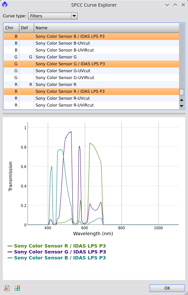
You can always select a QE curve and a filter set similar to the ones you have used to acquire the image. To know how those curves are, you can use the Curve Explorer dialog:

Here you will see the list of filters and camera sensitivity curves:
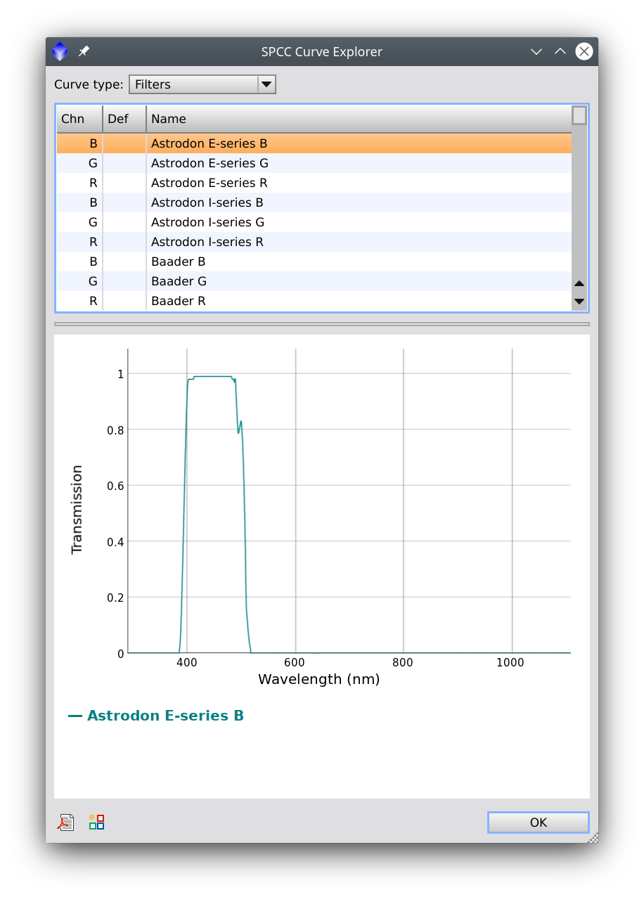
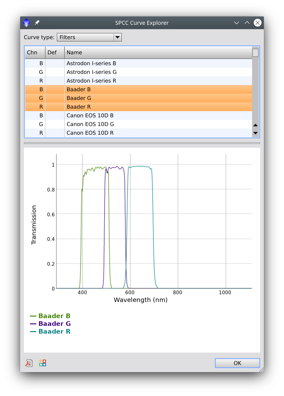
We can select any element in the list to visualize its curve. We can also select multiple elements in the list with the Control (Cmd in macOS) or Shift keys. For instance, in the figure below, we choose to visualize the Baader RGB set:
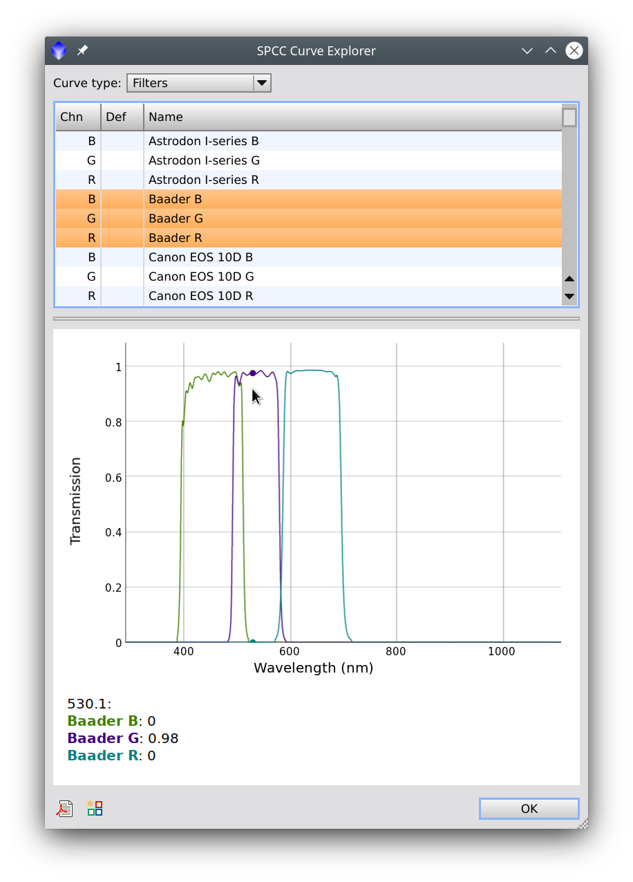
If we move the mouse over the graph, we'll get the wavelength and curve readouts:
The same applies to the camera sensitivity curves (or quantum efficiency curves), which are marked with a Q in the first column of the list:

By analyzing these curves, it's easy to decide which ones are the most similar to the equipment we're using. But we can also import our own filters by using the Filter Management dialog.
6.1 Narrowband Working Mode
We can configure SPCC to work with narrowband images. We do this by checking the Narrowband filters mode checkbox:

In narrowband mode, the filter selection controls are replaced with fields where we can define the central wavelength and width of each narrowband filter we have used. By default, the values are for a HOO palette, where the H-alpha line goes to the red channel, and the [O III] line goes to the green and blue channels.
This is the configuration for a Hubble's palette using 3 nm filters:

Here is a list of the most common emission lines we use in astronomy:
- [S II]: 674.2 nm
- [N II]: 658.4 nm
- H-alpha: 656 nm
- [O III]: 500.7 nm
- H-beta: 486.1 nm
6.2 Background Neutralization
We can also apply a background neutralization with SPCC by activating the Background Neutralization section on the tool. It's essential to select the right background area, which we can do easily by creating a preview and dragging and dropping the preview selector tab on the Region of Interest area of the tool.
We discuss these parameters in depth in the Applying SPCC to Broadband Images section.
6.3 The Filter Management Dialog
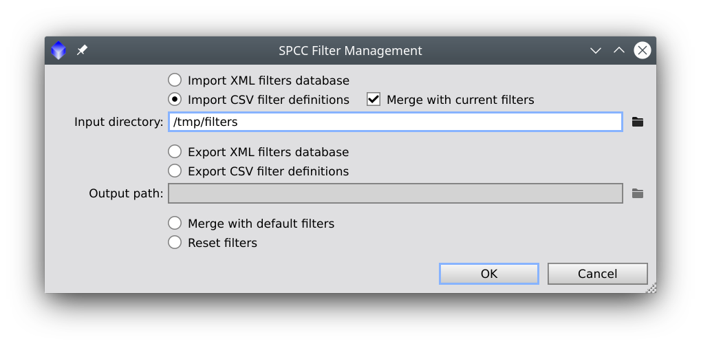
The SPCC process requires two special databases in XML format: one for white references and another for filter and quantum efficiency curve definitions. The white references database is part of the standard PixInsight software distribution and cannot be modified with the current implementation. However, the database where filters and QE curves are defined can be fully customized. The Filter Management dialog allows you to export, import and reset these curve definitions in several ways.
The dialog supports the following operations:
-
Import XML filters database
-
This option allows you to load filter and QE curve definitions from an existing database in XML format at the specified input path. Generally, you should have exported this file previously with the Export XML filters database option (see below) unless you can generate these databases on your own. If the Merge with current filters option is enabled, existing items (i.e., filters or QE curves with the same names as items being imported) will be replaced, and newly defined items will be created. If this option is disabled, the current filters and QE curves will be lost and replaced with imported ones.
-
Import CSV filter definitions
-
If this option is selected, you must select an existing input directory, where the process will search for CSV files (with the .csv file extension) with filter and/or QE curve definitions. The remarks regarding the Merge with current filters option we have made above for XML databases also apply in this case. The CSV files are expected to follow a straightforward format, which we describe in the next subsection. This option provides the most helpful way to customize your filter and QE curve collections.
-
Export XML filters database
-
With this option enabled, you have to select an output path, where the current set of filters and QE curves will be written in the special XML format used by the SPCC tool. You can import this database later with the Import XML filters database option, and you can select this database as the default one for the SPCC tool with the SPCC Preferences dialog.
-
Export CSV filter definitions
-
This option allows you to export the current set of filters and QE curves as individual files in CSV format (.csv file extension) on the specified output directory. This is useful in case you want to customize some of these files, or when you have created new ones. You can import these files later with the Import CSV filter definitions option.
-
Merge with default filters
-
Suppose you have imported a new database of filters and/or QE curves that you have customized or created, and then you want to use, along with them, the factory-default set. This option will merge the current filters and QE curves with the default database in the standard PixInsight distribution.
-
Reset filters
-
Select this option to replace the current filters and QE curves with the factory-default database of the standard PixInsight distribution.
6.3.1 CSV Curve Definition Format
The Filter Management dialog provides two options to import and export filter and QE curve definitions in CSV format. Each filter or QE curve must be defined in a separate file with the .csv file extension, which is expected to follow a very simple format we'll describe now.
CSV stands for comma-separated values.[29] SPCC filter definition CSV files are plain text files where each line contains two items separated by a comma (',') character. The first item is a field name, and the second is a field value. With several fields defined this way, a CSV file provides the necessary data to generate a filter's transmission curve or a quantum efficiency curve. The following fields are required:
Field name |
Field value |
|---|---|
type |
"filter" |
name |
"<filter-or-curve-name>" |
wavelength |
"<l1,l2,...,ln>" |
transmission |
"<t1,t2,...,tn>" |
The type field must always have the value filter in the current implementation. <filter-or-curve-name> represents the name of the filter or QE curve being defined, which can be any arbitrary text. However, we recommend avoiding too long or too complicated names, which can cause problems with their selection in curve and filter lists. In the wavelength field definition, <l1,l2,...,ln> is a comma-separated list of wavelengths expressed in nanometers. The list must specify a sequence of at least five distinct values sorted in ascending order. In the wavelength field definition, <t1,t2,...,tn> is a comma-separated list of filter transmission or sensitivity values in the [0,1] range. This list must have the same number of elements as the corresponding wavelength field definition.
The following two fields are optional:
Field name |
Field value |
|---|---|
channel |
one of: "R", "G", "B", "Q" |
default |
one of: "R", "G", "B", "Q" |
reference |
"<data-source-description>" |
If a supported channel field value is specified, the curve will be included exclusively in the red filter, green filter, blue filter or QE curve list, respectively for the field values R, G, B and Q. This is useful when a filter corresponds to one of the primary colors, or when a QE curve is being defined. If no channel field is specified, the curve will be included in the three red filter, green filter and blue filter lists. This is useful for filters that cannot be associated with a particular primary color, such as some standard photometric filters. Finally, if the specified channel field value is not one of R, G, B or Q, the curve won't be included in SPCC's drop-down selection lists, although it will be visible in the Curve Explorer dialog.
If a supported default field value is specified, the curve will be the one selected by default in the corresponding drop-down list of the SPCC tool window.
The reference field allows you to include information on the source of the data used to generate the CSV file. This field is typically used to specify the URL of a website or service where filter or QE curve data have been retrieved.
Let's see an example of an actual CSV filter definition file to better understand how this format works:
type,"filter"
name,"Sony Color Sensor R-UVIRcut"
channel,"R"
default,"R"
wavelength,"400,402,404,406,408,410,412,414,416,418,420,422,424,426,..."
transmission,"0.088,0.084,0.080,0.076,0.072,0.068,0.065,0.061,0.058,..."
In this example, we have abbreviated the long lists of wavelength and transmission values with ellipsis characters for simplicity. As you can see, this is the definition of the Sony Color Sensor R-UVIRcut filter, which is a red filter and the default filter for the red channel.
In the following example we define the QE curve of a Gpixel GSENSE2020BSI CMOS image sensor:
type,"filter"
name,"GSENSE2020BSI"
channel,"Q"
reference,"https://www.gpixel.com/"
wavelength,"204,206,208,210,212,214,216,218,220,222,224,226,228,230,..."
transmission,"0.1697,0.189,0.2083,0.2275,0.2468,0.2661,0.2853,0.3046,..."
6.4 The SPCC Preferences Dialog

To open the SPCC Preferences dialog, click the Preferences button on the SPCC tool window. As is customary in PixInsight, this button has a wrench icon and is located at the bottom right corner of the SPCC window, just before the Reset button.
As you see above, SPCC preferences are pretty simple: they just allow you to select a default XML filter and QE curve database with the .xspd file extension, which stands for eXtensible SPectrum Database. Although describing the details of this XML–based format is too advanced for the scope of this document, you need to use .xspd files in case you want to customize your filter or QE curves. We can describe the basic customization procedure as follows:
- Open the Filter Management dialog and export the current filters and QE curves as CSV files.
- Customize one or more filters or QE curves by editing the corresponding .csv files, and/or remove unnecessary ones by deleting .csv files.
- Import the customized CSV files from the Filter Management dialog, optionally merging them with the current set.
- With Filter Management, export the current filters and QE curves as an XML database. This will create a new .xspd file.
- Use the SPCC Preferences dialog to select the newly created .xspd file. From now on, this file will define the default set of filters and QE curves in the SPCC tool.
On the SPCC Preferences dialog, you can also restore the factory–default filters and QE curves by clicking the Default Filters Database button. In such a case, be aware that the current set will be replaced, and any unexported changes will be lost.
7 Applying SPCC to Broadband Images
[hide]
7.1 Monochrome Cameras
To calibrate a color image from a mono camera, we should always first compose the color image with ChannelCombination. In each channel, we import the three linear master light images for each filter:

Once we apply this process globally, a new color image is created in the current workspace. If the master images have an astrometric solution, ChannelCombination will copy it to the newly created color image if we have the Inherit astrometric solution option enabled.
As usual, the resulting image will have a completely random color, mainly because of the changing background sky brightness on each channel. Please remember to deactivate the Link RGB Channels[30] button and click the Auto Stretch button in the STF tool before performing the color calibration to have a better on–screen visualization of the uncalibrated image:


Please keep in mind that while the STF AutoStretch visualization with unlinked RGB channels is way better, this image does not provide an accurate color representation since each primary color is being stretched differently. An accurate color representation is only possible after performing a color calibration process and stretching the three primary colors exactly in the same way.
Provided we have a linear color image with a valid astrometric solution, we can perform the color calibration with SPCC. The filters and the white reference are the two main parameters we have to configure in this tool. In the case of this image of NGC 281, we select the default average spiral galaxy as the white reference. Then we choose the filters we used to acquire each primary color. Selecting the camera's QE curve will increase the robustness of color calibration. If you don't find your exact camera model in the list, you can choose the default Ideal QE curve option, which will consider that the camera is equally sensitive throughout the entire spectrum. Alternatively, you can select a QE curve that approximates the spectral sensitivity of your camera. You can take a look at the available curves with the Curve Explorer dialog. You can see below the configuration of SPCC for the current image:
Finally, if we want to correct the sky background level, we should enable the Background Neutralization section. Please remember that the background reference area can be easily configured by creating a preview, then dragging and dropping the preview selector over the Region of Interest area of the tool's interface.[31]
Once we execute the process, if the Generate graphs option is enabled, SPCC opens the White Balance Functions window:
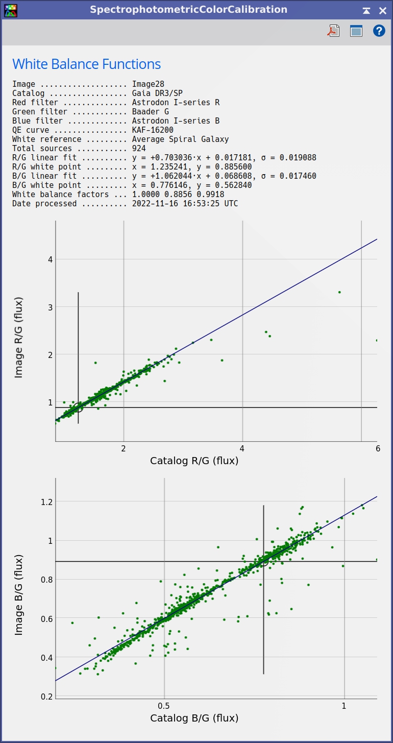
One should always check that the fitted lines adequately follow the measured points and the overall shape of the point clouds. If we find a higher–than–usual dispersion, it can be due to strong multiplicative gradients present in our image, primarily due to a wrong flat field correction. It's also important to point out that color calibration will be more accurate if the white reference (signaled by two cross lines in each graph) is well within the point cloud and in its linear range. As we'll see below, under some circumstances, the image–to–catalog color relationship won't be wholly linear, but in any case, we have been extremely careful to implement the best possible linear fitting algorithm. This algorithm ensures the maximum robustness to protect the process against this kind of outliers.
If needed, we can zoom the graphs in horizontal or vertical directions. In this case, we can zoom horizontally on the upper graph. We do this by clicking on the graph and dragging the cursor horizontally over the area of interest, as shown in the figure below. The graph will then show only the selected area:

After performing the color calibration, please link the RGB channels[30] in STF and click the Auto Stretch button again. Only with these settings can we visualize the actual color calibration we have just performed. No other settings can work adequately to evaluate this process. This is also true for the image stretching process with histograms: the stretching should be applied always in the same way to the three color channels. Otherwise, you'll destroy the calculated color balance.
After readjusting the STF visualization, we get this color–calibrated image:
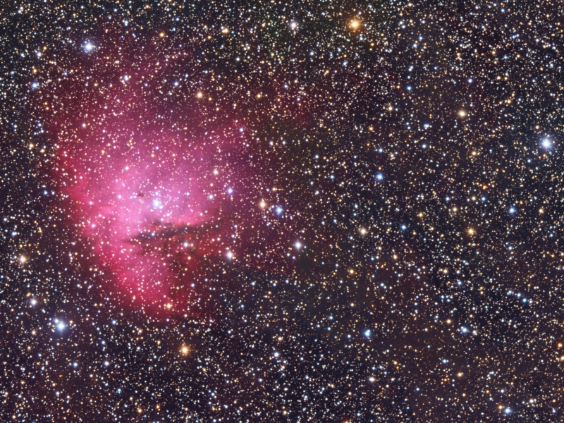
Image by Vicent Peris (OAUV), Alicia Lozano, OAUV, OAO.
7.2 One–Shot Color Cameras
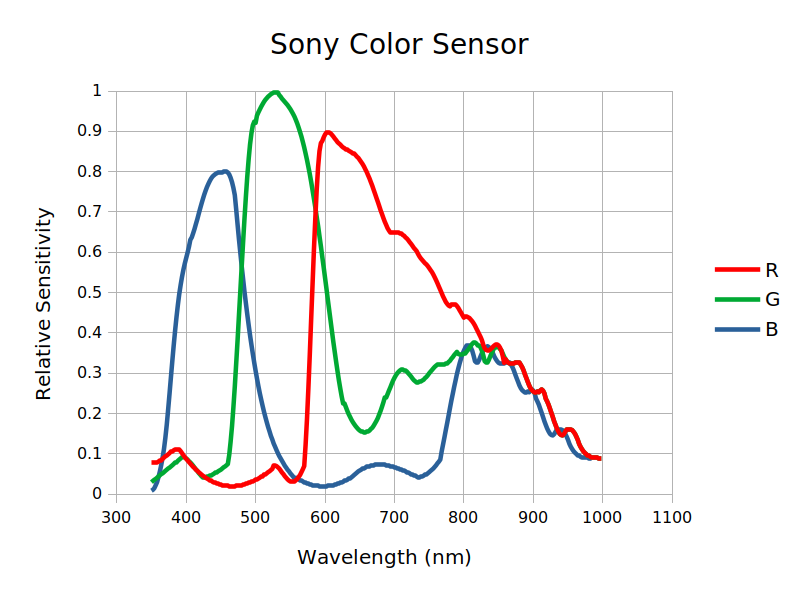
In the case of color cameras, we have a generic set of RGB filters for Sony color sensors (both CCD and CMOS). There are three options for these sensors:
- Sony Color Sensor. Full sensitivity range of the sensor, from ultraviolet to infrared.
- Sony Color Sensor UVcut. Sensitivity range starting at 400 nm, rejecting the ultraviolet but including the infrared.
- Sony Color Sensor UVIRcut. Sensitivity range including only the visual spectrum, from 400 to 700 nm, thus rejecting both the ultraviolet and infrared ranges.
We strongly recommend using a camera system that rejects ultraviolet and infrared light. This can be done using the right camera optical window or a UV/IR cut filter. Although this decreases the total light gathered by the camera, the resulting color will be much more accurate because the RGB sensitivity curves are completely mixed in the infrared range, as seen below:
Below we can see a color–calibrated image of Messier 33, acquired with a camera equipped with a Sony ICX694AQG CCD color sensor:

Image courtesy of Constantino Rodas.
The Sony color sensor curves include the quantum efficiency curve implicitly. Therefore, when working with OSC cameras, we should always set the QE curve parameter to Ideal QE curve, as shown below:
Another important point when working with OSC cameras is to always use drizzle. Besides the fact that only a drizzle integration can provide optimal results by avoiding interpolation, some de-Bayering algorithms may modify color proportions at small scales, where interpolation of missing color data in CFA patterns plays an important role. This is the case with VNG. While large–scale structures remain untouched, point sources (like stars) will be altered. And, what is worse, this color shift depends on the sizes of the stars so that each image can be altered differently. This affects stellar photometry so that de-Bayering can lead to unexpected erroneous results, both with PCC and SPCC. You can see two examples below; the first one is with the same Messier 33 image used previously:

The same happens with this image of M31, shot with a Sony IMX294 CMOS color sensor:

Image courtesy of Federico Boninsegna.
7.3 Broadband Calibration Examples
Image by Vicent Peris (OAUV), Alicia Lozano, OAUV, OAO.
If we zoom into the NGC 6946 image above, we can see that the resulting color calibration shows the reddening of the spiral galaxy, which is located very near to the galactic plane:
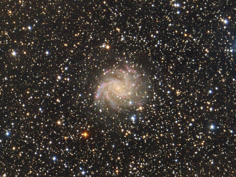
Image by Vicent Peris (OAUV), Alicia Lozano, OAUV, OAO.
Another good example of galactic dust reddening is the spiral galaxy IC342, here calibrated with the average spiral galaxy white reference:
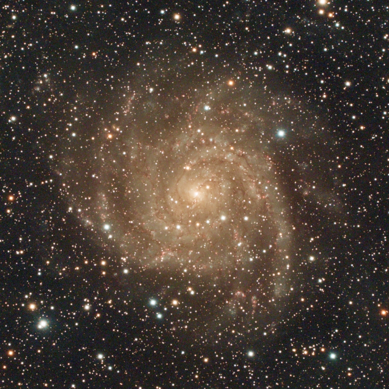
Image courtesy of Alessandro Bianconi.
This image was acquired with a Sony IMX571 CMOS color sensor and an IDAS LPS P3 filter, so we combined these filters with Curve Explorer:
In PixInsight, we have always favored a relativistic view of color in astrophotography. This is well described in the book Fotografiar lo invisible,[32] by Vicent Peris:
From this point of view, an image can have multiple color perspectives, depending on the natural content we want to convey. The Messier 81 and Messier 82 galaxy pair is an interesting example. The image below was calibrated using the average spiral galaxy as the white reference:
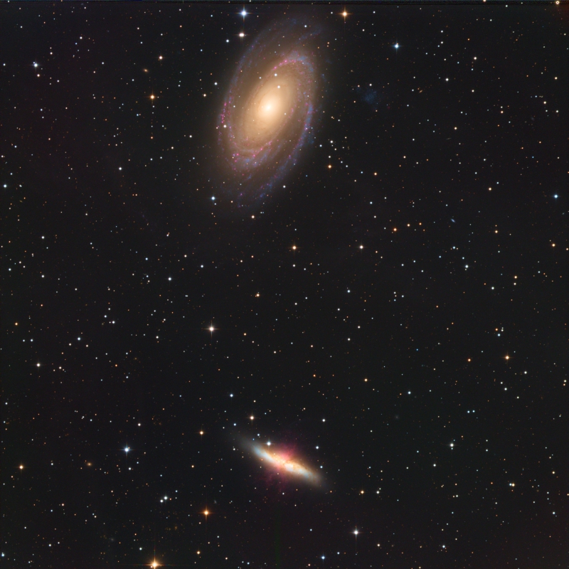
Image courtesy of Bob Rieger.
We can also tune the color balance to the morphological type of Messier 81: Sb. In this way, we neutralize the reddish cast inside this galaxy:

The same concept can be applied to the Virgo Cluster image shown below:
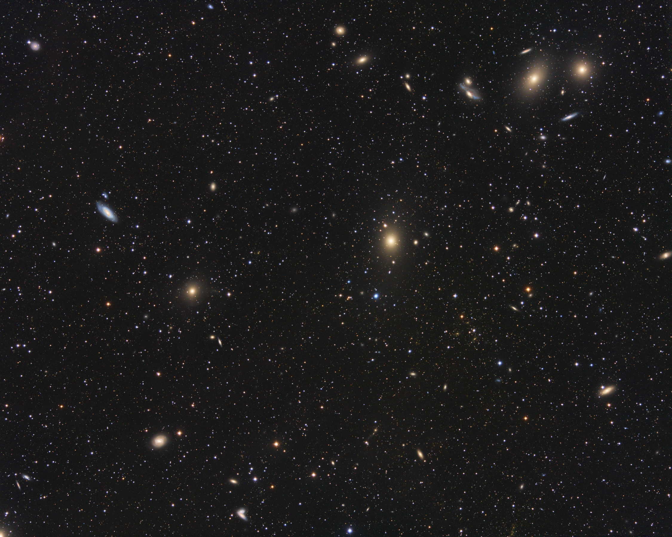
Image by Vicent Peris (OAUV), OAUV, OAO.
This image was calibrated using the average spiral galaxy as white reference. In this case, the selected reference works very well because it optimizes the differentiation among stellar populations in these galaxies. But we can also change the white balance to an elliptical galaxy to neutralize the color of Messier 87:
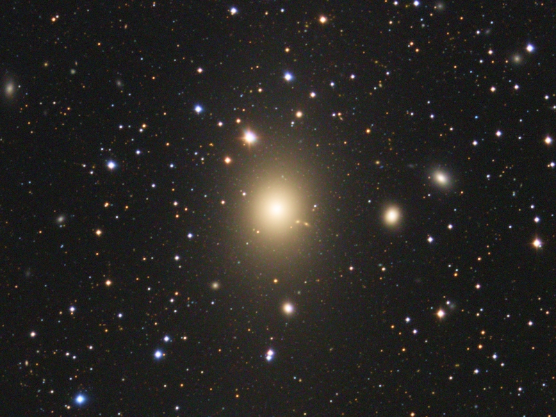
This is good proof of the accuracy of the photometry that we are using as the elliptical galaxy becomes white. And this allows us to see tiny differences in color between multiple elliptical galaxies. For example, the small elliptical galaxy to the right of Messier 87 is clearly bluer. Below you can see some crops around the elliptical galaxies in this picture:
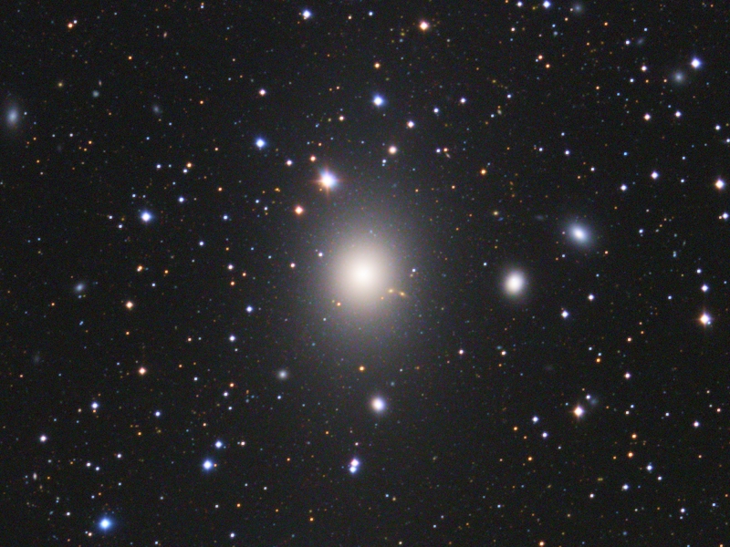
The color differences are very subtle since all the hues are close to the white reference, but this rendition shows that each elliptical galaxy has its specific color.
We can also tune the white balancing to a specific star spectral type. In the NGC 7023 picture below, we used the average spiral galaxy as white reference. This calibration shows very well the usual bluish reflection nebulae:
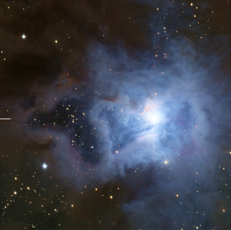
Image by Vicent Peris (OAUV), Jack Harvey (SSRO), Steve Mazlin (SSRO), Fundación Descubre, CAHA, DSA, OAUV.
We can also calibrate the color by selecting as white reference the spectral type of the central star: B2V. Since we don't have this spectral type in SPCC, we choose the closest one available: B3V. If we zoom into the bright central star, the resulting image shows something exciting:
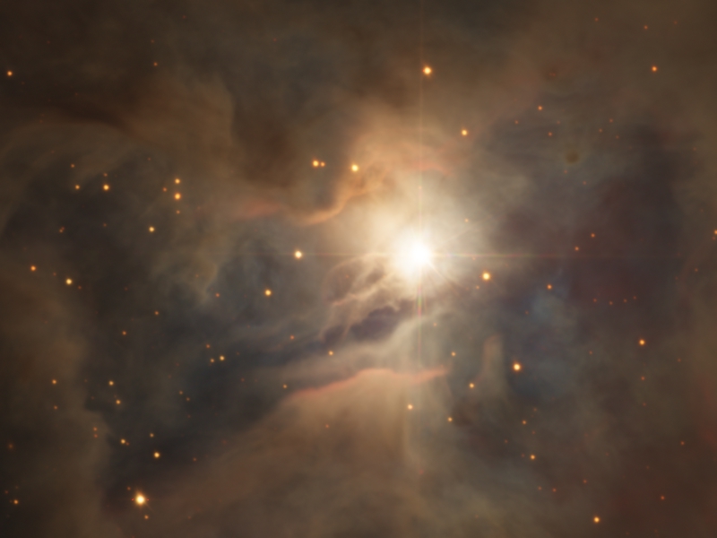
Instead of becoming white like in the previous example, the star remains yellowish this time. What we are looking at here is the reddening of the central star by the dust between the star and us.
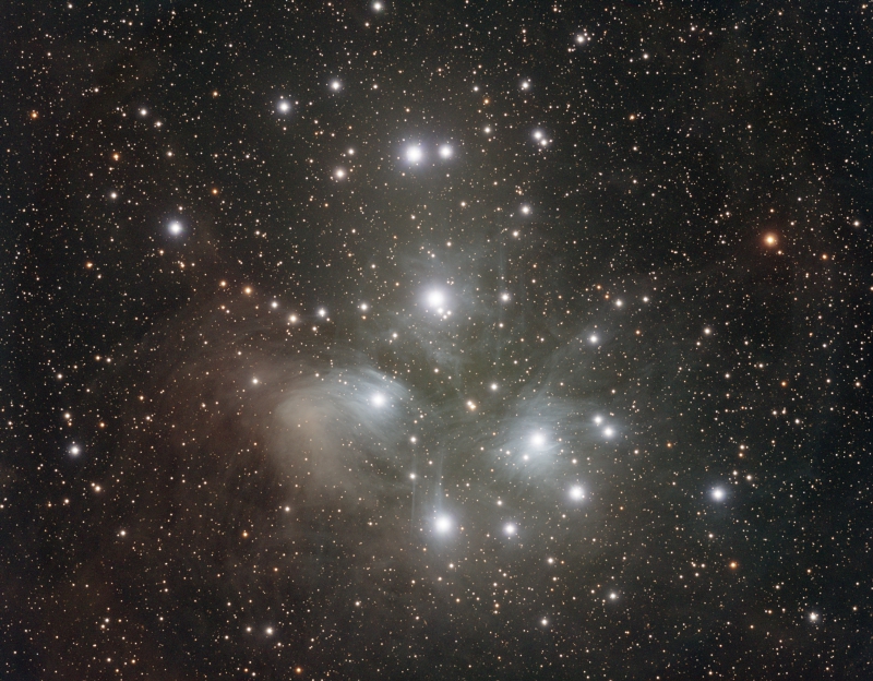
Something similar happens with this picture of the Pleiades, calibrated below with the average spiral galaxy as white reference:

Image courtesy of Edoardo Luca Radice.
When we change the white reference to the average spectral type of the main stars of the cluster, the blue–colored clouds become white. We can then better differentiate the brown clouds in the area:
8 Applying SPCC to Narrowband Images
[hide]
The narrowband working mode in PCC has been discontinued since the narrowband emission lines can be calculated with much more accuracy in SPCC. This is because SPCC calculates the brightness of each measured star exclusively within the small interval of wavelengths transmitted by narrowband filters. Thus, we no longer need to rely on imprecise star brightness comparisons between broad and narrowband filters.
The most common case is an image where we assign the H-alpha filter to the red channel and the [O III] to the green and blue channels (HOO composition). In this case, the first step is to create a color image with ChannelCombination by assigning each narrowband master image to its corresponding color channel:

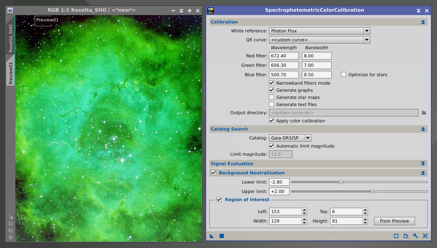
To calibrate the color of this image, we enable the Narrowband filters mode option in SPCC. Then, we should fill the filter data: center wavelength and bandwidth. By default, this is set to H-alpha wavelength in R and [O III] wavelength in G and B, all three filters being 3 nm wide.
Since we want an image where the intensity of the nebula in the different filters corresponds to the actual proportions between the emission lines, the white reference in this mode should be set to Photon Flux. Below you can see some examples.
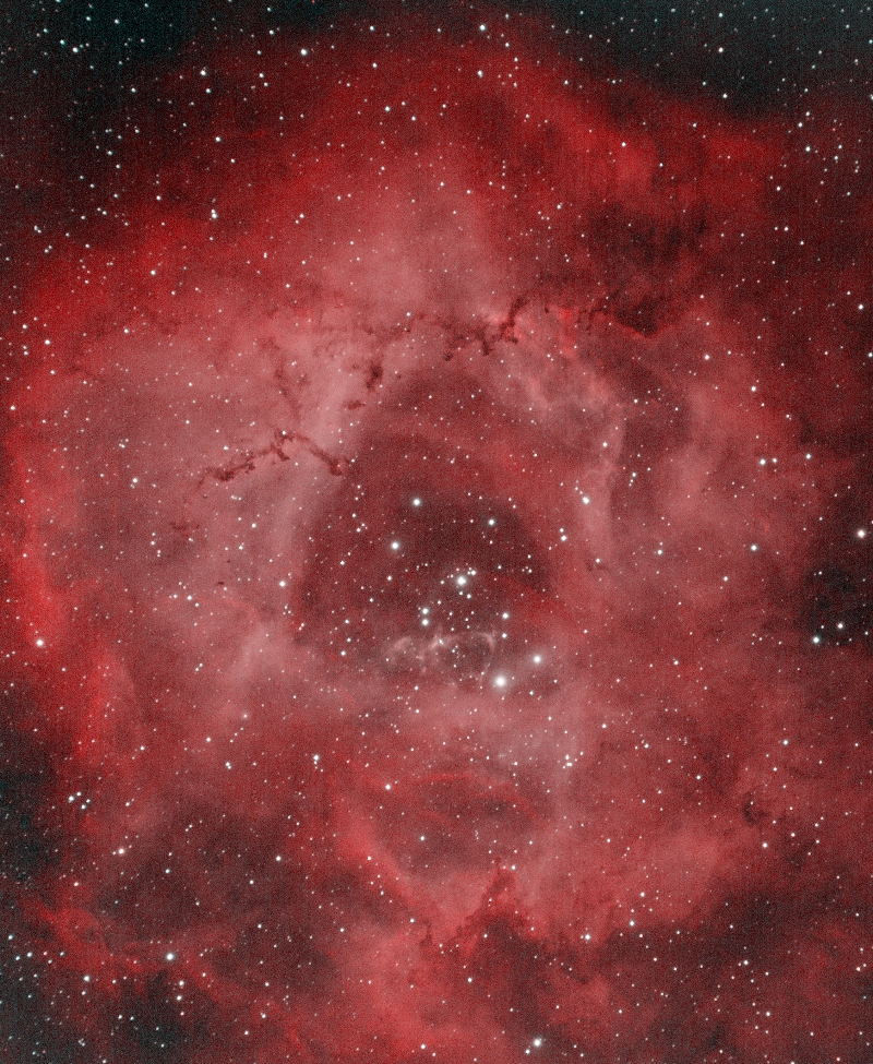
The Rosetta nebula (HOO composition). Image courtesy of Alicia Lozano.
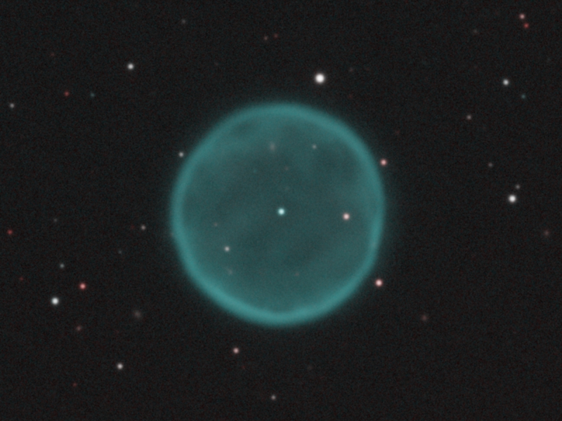
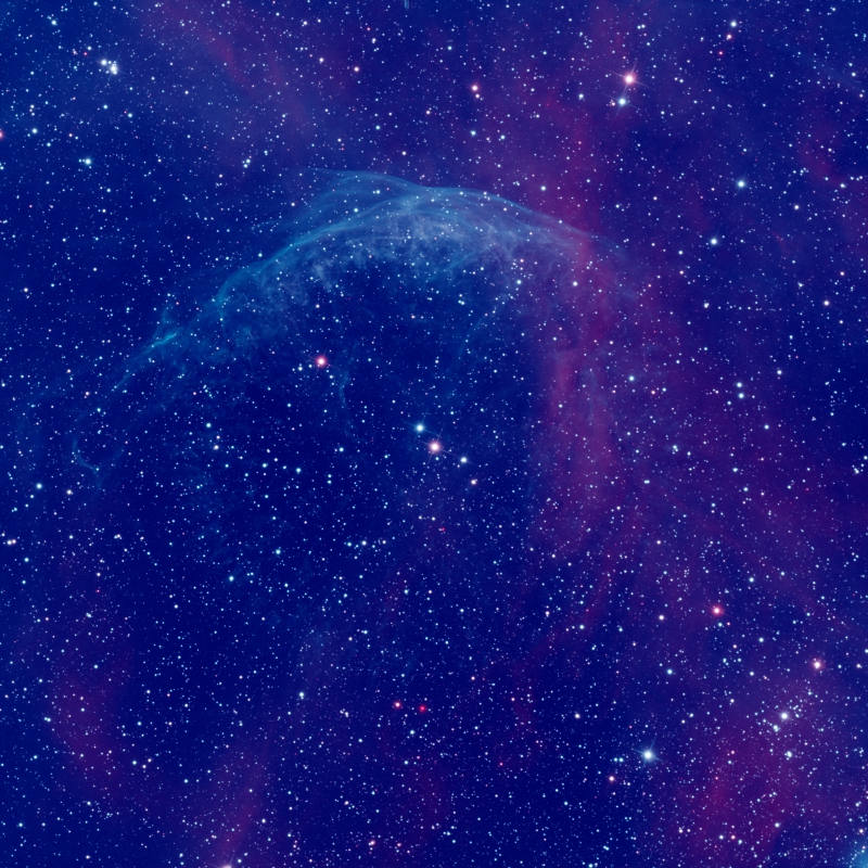
Abell 39 (HOO composition). Image by Vicent Peris (OAUV), OAUV, OAO.
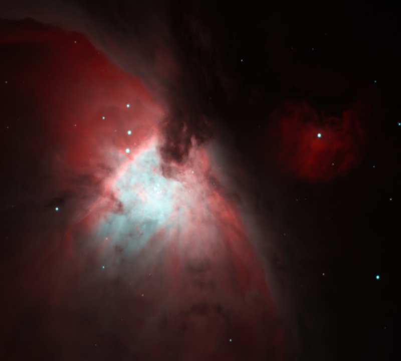
M42, the Orion nebula (HOO composition). Image by Vicent Peris (OAUV), OAUV, OAO.
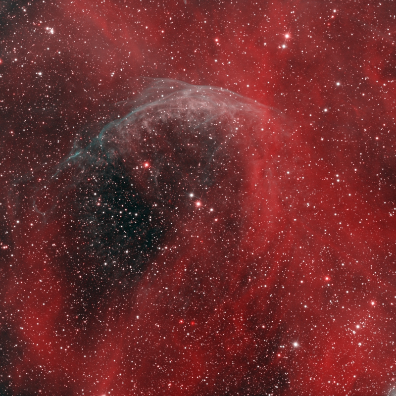
WR134 (HOO composition). Image by Vicent Peris (OAUV), Alicia Lozano, OAUV, OAO.
In some cases, the difference from the original image can be subtle. Still, the critical point here is that we know that the proportion between the emission lines in the processed image corresponds to reality. This is a main goal by itself, but we can also use it as a starting point to modify the color palette. For instance, in the WR134 image, we can vary the balance between G and B in [O III] to give this emission line a different hue. If we multiply the G channel by 0.6666 and the B channel by 1.3333, we'll shift the [O III] emission towards the blue since it will be twice more intense in this channel:

Then, if we want to uncover the delicate [O III] emission from inside the strong H-alpha emission, we can multiply [O III] by a factor of 2 by multiplying it in the G and B channels with PixelMath:
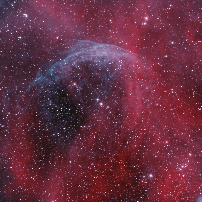
Since SPCC gave us a precise starting point, we can now say that the color mapping of this image has been done by placing the H-alpha in the red channel and the [O III] in green and blue with a proportion of 1:2, then enhancing the [O III] component by a factor of 2 with respect to H-alpha.
Remember that all these steps will require a final background neutralization; we can use the same preview we configured in SPCC for this task. This is the final image before and after the background neutralization process:
It is important to point out that a Hubble's palette configuration in SPCC will always give a poorly optimized color rendition. To apply this palette, we first create a color image with ChannelCombination. We assign the S-II image to the red channel, H-alpha to green, and [O III] to blue:

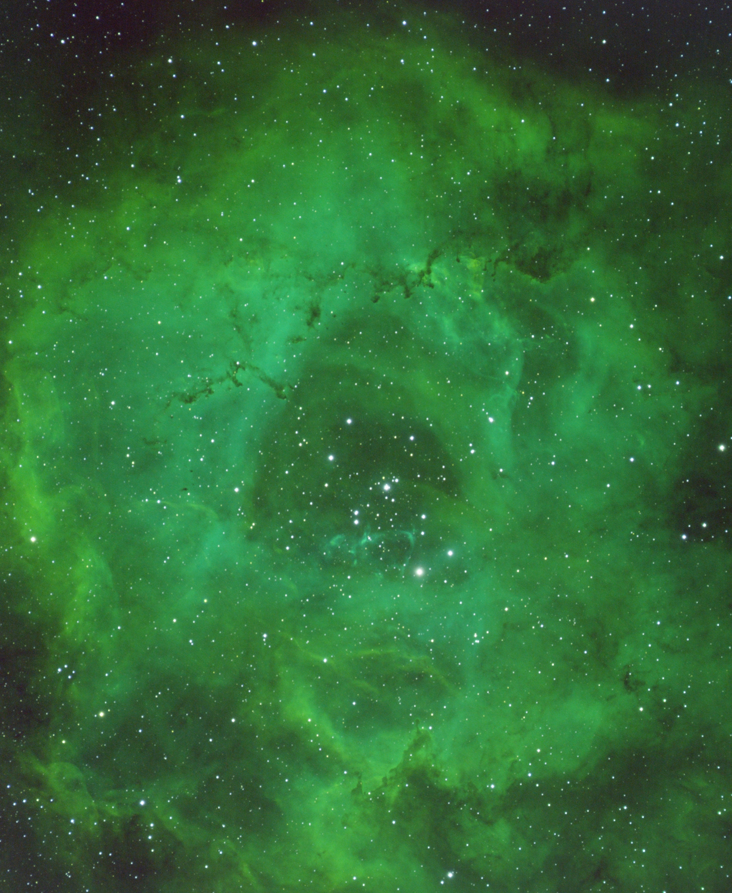
This is the result of applying SPCC to an SHO version of the Rosetta nebula picture:
The result will always look similar when using SPCC for this application. This happens because the S-II emission line is usually much weaker than the H-alpha and [O III] ones. To achieve a good Hubble's palette representation, we recommend using the ColorCalibration tool instead:
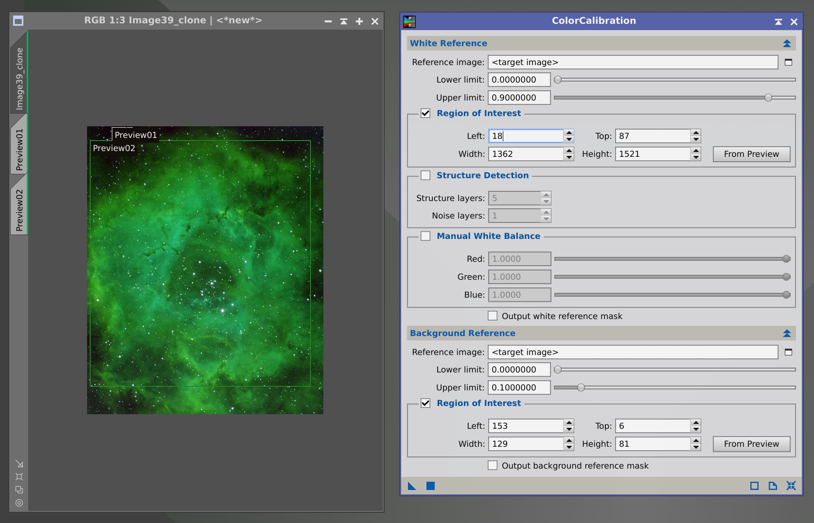
In ColorCalibration, we use the entire nebula as the white reference because we want to balance the intensity between the three emission lines. Note that the Structure detection checkbox has been disabled to sum all the light inside the preview; if we leave it checked, ColorCalibration will balance the color of small structures, that is, the stars, which is not what we want in this case.
Below you have two comparisons between SPCC and ColorCalibration results for SHO compositions:
The Rosetta nebula (SHO composition). Image courtesy of Alicia Lozano.

M42, the Orion nebula (SHO composition). Image by Vicent Peris (OAUV), OAUV, OAO.
Note that this is not a limitation of SPCC but a limitation imposed by the nature of the objects, requiring a different use of our color calibration tools.
9 On the Meaning of Color in Astrophotography: Best Practices
[hide]
In the PixInsight Development Team, we do think that the artwork of astrophotography is based on the unification of the inner pictorial content of the image with the documentary content of the scene. This defines the aesthetics of astrophotography, which lies at the point where beauty meets authenticity.[33]
At this point lies SPCC, whose goal is to materialize the above philosophy in the work of art. The color calibration process provides a documentary value to the picture that cannot be undervalued, invalidated, or manipulated in the subsequent operations we apply to the image. This includes arbitrary manipulation of individual hues, incorrect use of the delinearization processes, arbitrary use of the RGB curves, or applying any color transformation process without having a rational documentary argument at its roots. Color calibration gives color meaning by itself in the picture; hence, we should preserve it up to the end of the creative process.
A few processes that can break the meaning of color in the image are:
- A histogram transformation that changes each color channel separately.
- A curves transformation that changes each RGB channel separately.
- A curves transformation that changes the hue curve to arbitrarly modify the hues in the image.
- A curve applied through ColorSaturation to selectively enhance specific hues.
- SCNR applied to remove green tones from the image.
10 Conclusions
[hide]
When we designed the PCC tool, we thought it was a temporary solution for the color calibration task. At that moment, PixInsight had only color calibration techniques that were intrinsic to the image, in the sense that it was required to select the white reference inside the image. PCC provided us with the first extrinsic color referencing, and more importantly, it used the first photometric catalog built with modern imaging techniques: the APASS catalog. Moreover, one of the primary goals in the design of the AperturePhotometry script was to provide PixInsight with the ability to perform photometric measurements of the stars, which was absolutely lacking in the platform then. For these reasons, both the AperturePhotometry script and the PCC tool were the perfect test workbench to demonstrate that photometry, along with modern star catalogs, would be the needed platform to allow us to materialize our new philosophy of color: the definition of a new astrophotography color referencing standard based on a spiral galaxy instead of the sunlight. This, obviously, can only be done through star color measurements with photometry, since you cannot have a face–on spiral galaxy in every image.
The success of the implementation of SPCC is due to two decisive features of the PixInsight platform. First is the adequate use of the gigantic database that allows us to access 80 billion data in milliseconds. Second, the new hybrid photometric engine (the same that has been implemented in the LocalNormalization tool) outperforms the capabilities of the AperturePhotometry script in both precision and resource optimization. Both PCC and SPCC run now much faster and more accurately.
PCC was a temporary solution for us because we were waiting for the release of the Gaia spectrophotometric catalog. We knew this catalog would be the definitive solution for our needs. Now, PCC and APASS will be deprecated in most use cases, and we do think SPCC will be the flexible, precise and accurate tool we'll need in the upcoming years. Therefore, SPCC represents the culmination of nearly ten years of work.
11 Acknowledgments
[hide]
- Gaia DR3
-
This work has made use of data from the European Space Agency (ESA) mission Gaia (https://www.cosmos.esa.int/gaia), processed by the Gaia Data Processing and Analysis Consortium (DPAC, https://www.cosmos.esa.int/web/gaia/dpac/consortium). Funding for the DPAC has been provided by national institutions, in particular the institutions participating in the Gaia Multilateral Agreement.
- GaiaXPy
-
This job has made use of the Python package GaiaXPy (https://gaia-dpci.github.io/GaiaXPy-website/), developed and maintained by members of the Gaia Data Processing and Analysis Consortium (DPAC), and in particular, Coordination Unit 5 (CU5), and the Data Processing Centre located at the Institute of Astronomy, Cambridge, UK (DPCI).
References
[1] AAVSO website: APASS: The AAVSO Photometric All–Sky Survey
[2] Gaia Collaboration, T. Prusti, J.H.J. de Bruijne, et al (2016b). The Gaia mission. Astronomy & Astrophysics 595, pp. A1.
[3] ESA website: the Gaia Archive at ESA
[4] Gaia Data Release 3 Documentation: 5.3.6 Catalogue of BP/RP spectra in Gaia DR3
[5] Gaia Collaboration, A. Vallenari, A. G. A. Brown, et al (2022k). Gaia Data Release 3: Summary of the content and survey properties. arXiv e-prints, pp. arXiv:2208.00211.
[6] ESA website: Gaia Data Release 3
[7] ESA website: Gaia DR3 Papers
[8] V. Peris and J. Conejero (2015). ALHAMBRA Survey: RGB Image Synthesis
[9] Vicent Peris (2020). Fotografiar lo invisible. La estética de la astrofotografía. El arte naturalista en el siglo XXI., pp. 164-178
[10] Mari Polletta's web site: SWIRE Template Library
[11] Polletta et al (2007). Spectral energy distributions of hard X-ray selected AGNs. The Astrophysical Journal, 663, 81.
[12] Strasbourg Astronomical Data Center website: The VizieR Catalogue Service
[13] J. Conejero (2017). XISF Version 1.0 Specification
[14] PCL documentation: Star Catalogs and Point Source Databases
[15] Wikipedia article: Levenberg–Marquardt algorithm
[16] Moffat, A. F. J. (1969). A Theoretical Investigation of Focal Stellar Images in the Photographic Emulsion and Application to Photographic Photometry. Astronomy and Astrophysics, Vol. 3, p. 455
[17] J. Conejero (2019). New Plate Solving Distortion Correction Algorithm in PixInsight
[18] Mark de Berg et al (2010). Computational Geometry: Algorithms and Applications (3rd Edition). Springer. Chapter 14.
[19] Hanan Samet (2006). Foundations of Multidimensional and Metric Data Structures. Morgan Kaufmann. § 1.4.
[20] Sean Urban and P. Kenneth Seidelmann, Ed. (2013). Explanatory Supplement to the Astronomical Almanac (3rd Edition). University Science Books. Chapter 7.
[21] Ryan S. Park et al (2021). The JPL Planetary and Lunar Ephemerides DE440 and DE441. The Astronomical Journal, Vol. 161, No. 3
[22] Hiroshi Akima (1970). A new method of interpolation and smooth curve fitting based on local procedures. Journal of the ACM, Vol. 17, No. 4, pp. 589–602
[23] Gisela Engeln-Müllges and Frank Uhlig (1996). Numerical Algorithms with C. Springer. § 13.1.
[24] Wikipedia article: Simpson's rule
[25] Andrew F. Siegel (1982). Robust regression using repeated medians. Biometrika, 69(1): 242–244
[26] Peter J. Rousseeuw et al (1993). New Statistical and Computational Results on the Repeated Median Regression Estimator. New Directions in Statistical Data Analysis and Robustness, © Birkhauser Verlag, Basel, pp. 177–194
[27] Rand R. Wilcox (2022). Introduction to Robust Estimating and Hypothesis Testing, Fifth Edition. Academic Press. © 2022 Elsevier Inc. All rights reserved. § 3.4
[28] William H. Press et al (2007). Numerical Recipes, The Art of Scientific Computing, 3rd Ed. Cambridge University Press, § 15.7.3, pp. 822–824
[29] Wikipedia article: Comma-separated values
[30] PixInsight Official YouTube channel: Introduction to PixInsight — 08 ScreenTransferFunction (Part 3)
[31] PixInsight Official YouTube channel: Introduction to PixInsight — 10 Process Windows (Part 1)
[32] Vicent Peris (2020). Fotografiar lo invisible. La estética de la astrofotografía. El arte naturalista en el siglo XXI., p. 175
[33] Vicent Peris (2020). Fotografiar lo invisible. La estética de la astrofotografía. El arte naturalista en el siglo XXI., p. 201
Copyright © 2022 Pleiades Astrophoto. All Rights Reserved.