ALHAMBRA Survey - RGB Image Synthesis Examples

Filter Sets

For RGB image synthesis with the 23 ALHAMBRA filters we construct a filter set consisting of individual red, green and blue filters, which we define by the following equation:

This function returns the filter weight in the [0,1] range for a given wavelength x. The function parameters are as follows:

• c : Central wavelength.
• w₁ : Filter width, left side, in wavelength units.
• w₂ : Filter width, right side, in wavelength units.
• s₁ : Shape parameter, left side, 0 < s₁.
• s₂ : Shape parameter, right side, 0 < s₂.

The shape parameters control the geometry of the filter's profile in terms of its kurtosis:

• s = 2 : Gaussian
• s < 2 : Leptokurtic (peaked filter)
• s > 2 : Mesokurtic (flat filter)

This function allows us to model each filter separately with great accuracy and flexibility. Four filter sets have been defined in this example, which we have called extended, uniform, dense and visual, respectively for easy identification.

Extended filter set

This set aims at representing the whole data set available, while providing a plausible visual color representation.

Uniform filter set

This set covers only the main data subset uniformly with Gaussian filter shapes.

Dense filter set

Covers only the main data subset uniformly with flat filters.

Visual filter set

Covers only the main data subset partially, with filters roughly centered at visual perception maxima.

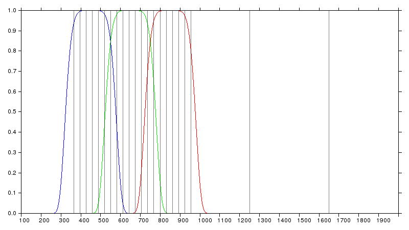
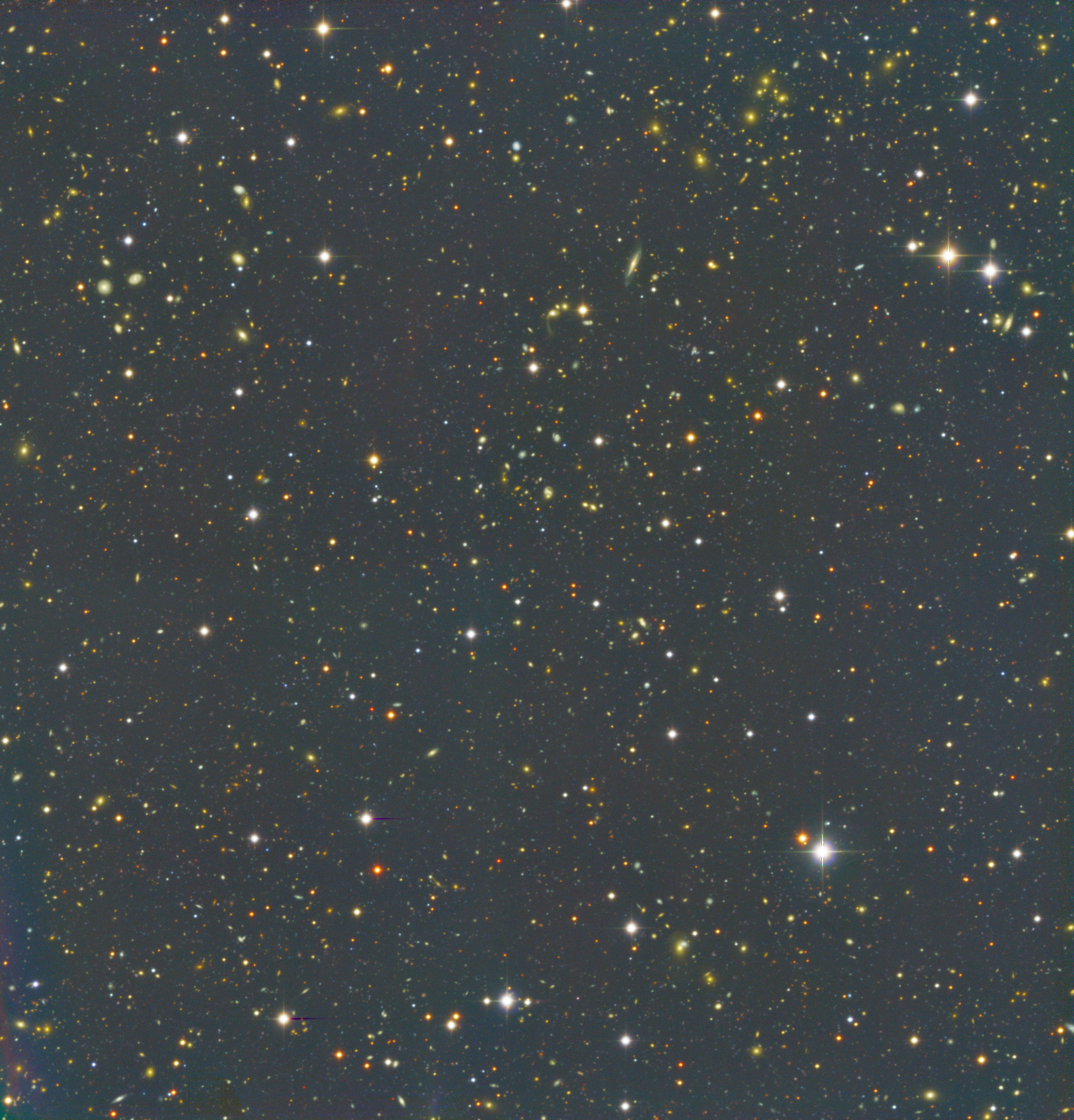
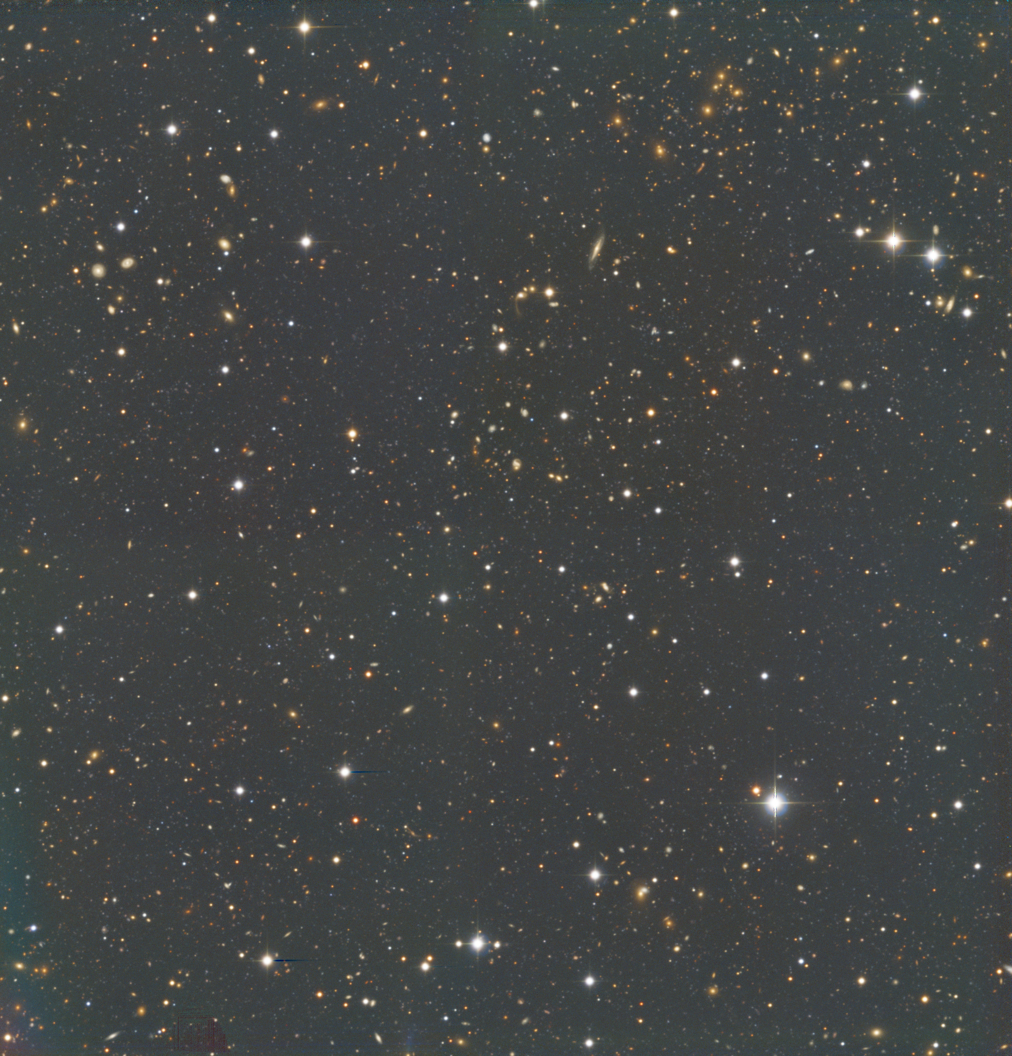
The filter functions and their parameters are represented and tabulated in the figures below. In each graphs of these figures, the horizontal axis represents wavelength in nm, and the vertical axis represents filter transmissivity. The vertical gray lines indicate the positions of the 23 ALHAMBRA filters (except the last K filter (2200 nm), which is not represented).

Crucial to achieve a good color rendition is having enough crossover between filters. Filter crossover is necessary to achieve rich and deep chroma components, where the red, green and blue components mix together to provide a continuous tonal representation without gaps.

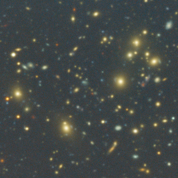
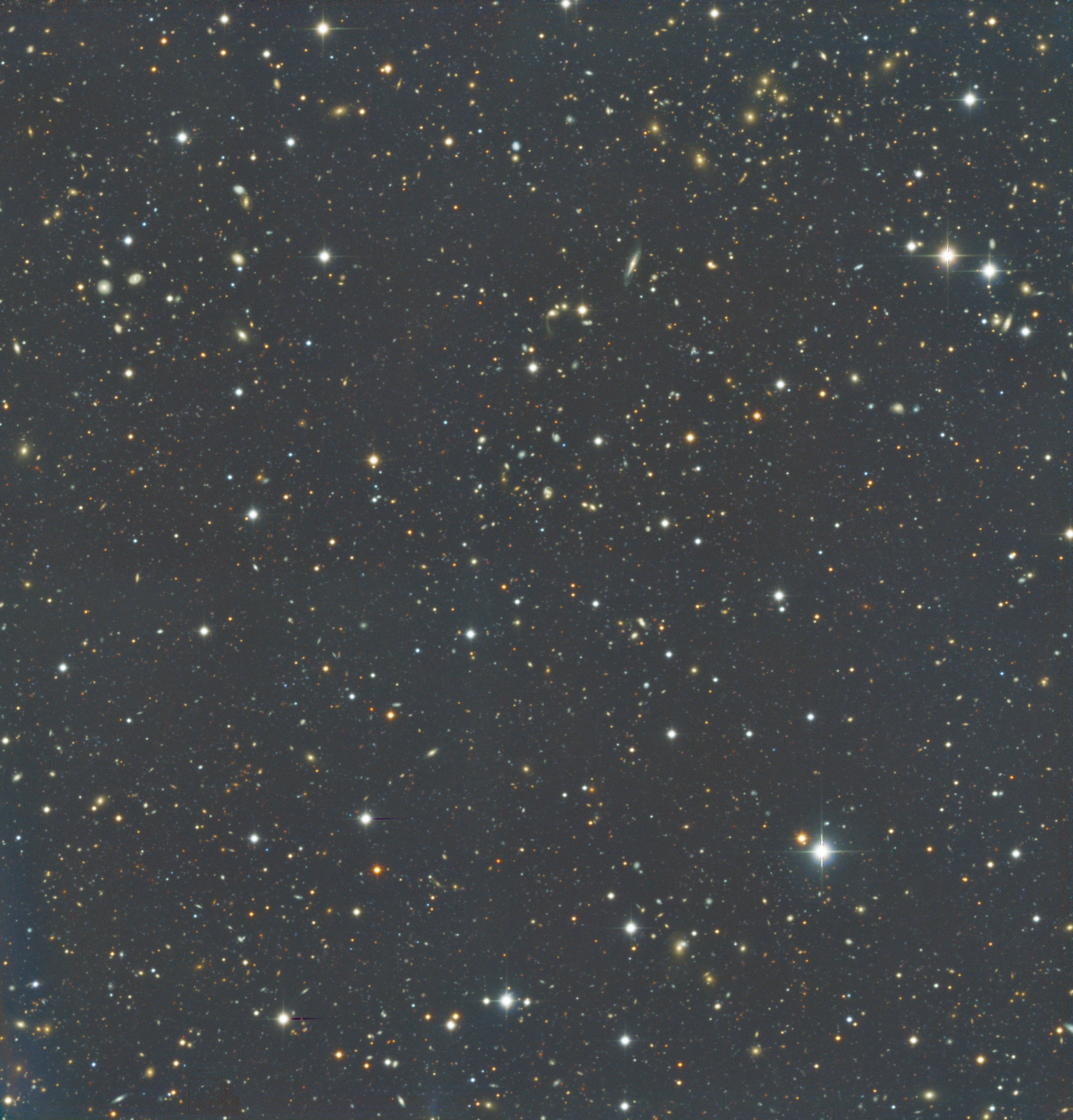
The whole work, including image synthesis and graph generation, has been performed in PixInsight with a JavaScript script that is available for download.

Image Comparisons

The following figures provide mouseover comparisons on selected crops of the full-size synthesized RGB images. The whole synthetic RGB images are also available for download:

• Extended filter set RGB image
• Uniform filter set RGB image
• Dense filter set RGB image
• Visual filter set RGB image