A New Approach to Combination of Broadband and Narrowband Data
Tutorial by Vicent Peris (PTeam)
Original raw data acquired by Jack Harvey, SSRO/PROMPT
Introduction
In this document I'll explain a new H-alpha / RGB combination method. I have developed this method with two priority goals: maximum H-alpha information preservation, and nonlinear star size control. These are the key features of this new algorithm:
- Fully controllable enhancement of line emission images.
- Accurate color representation of both line emission and continuum emission objects.
- Minimum signal-to-noise degradation in narrowband data.
- Effective star brightness reduction.
- Fully automatable workflow with consistent results.
Since the algorithm can be easily automated, it will be implemented as a PixInsight module as soon as possible.
In this article we'll talk about combination of H-alpha images with RGB data, but this technique can be applied to other emission lines as well. The future development of this method will include the combination of different narrowband and broadband images.
As I've said in the first paragraph, this method offers a solution to the two great problems that narrowband imaging has always had. We'll explain how to solve both problems in two separate sections.
This article is based on experiments made with an image of NGC 2074 acquired through H-alpha and RGB filters by Jack Harvey, of the Star Shadows Remote Observatory team (SSRO), from their location at the Cerro Tololo Inter-American Observatory (CTIO), in Chile. Many thanks to Jack for letting me use his raw data; this method wouldn't have been devised without his collaboration.
On Figure 1 you can see an example of the results that can be achieved with the algorithm described in this document.
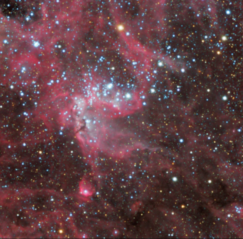
Figure 1— NGC 2074 HaRGB image obtained with the algorithm described in this article. Image processing performed in the PixInsight platform. Raw data acquired by Jack Harvey (SSRO/PROMPT) from CTIO (Chile) with a 16-inch RCOS telescope.
The original broadband data for this image is of exceptional quality. For demonstration purposes, a noisier version of the R image has been artificially created. As shown on Figure 2, a mix of synthetic Gaussian and Poisson noise has been added to the original linear image, which has allowed us to work with a simulation of broadband images acquired under more common (poorer) conditions.
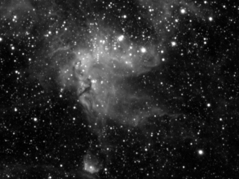
Figure 2— Adding synthetic noise to the original linear red image.
Mouseover: [Original R image] [Added Gaussian and Poisson noise]
The Problem of Having All Together
Several methods have been devised to combine H-alpha and RGB data with positive results. One approach consists of taking the result of a maximum operator applied to the H-alpha and red images. This operator yields the maximum value of each pair of pixels at the same coordinates. In this case, the maximum operator provides the correct star shapes and intensities, fixing well the luminosities of the fainter stars in the narrowband component.

Figure 3— Combination of the red and H-alpha components with the maximum operator.
Mouseover:
[Maximum of R and
(H-alpha + 0.001)]
As seen on Figure 3, the maximum operator works very well to fix star intensities, but it has an important drawback: it transfers a part of the noise from the broadband image to the otherwise immaculate narrowband image. On the other hand, the maximum operator won't work properly if the brightness and background illumination level in the narrowband image don't fit perfectly to the same properties of the broadband image.
Another approach consists of mixing both images, usually taking a higher contribution from the narrowband image. We illustrate this technique on Figure 4.
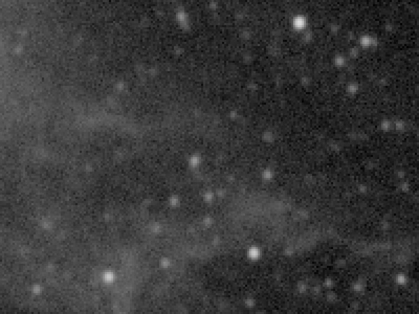
Figure 4— Mixing the red and H-alpha components at different combine ratios.
Mouseover:
Of course, this option is really bad as it doesn't provide a solution to anything: it doesn't recover the correct brightness of the stars, and it does degrade terribly the signal-to-noise ratio of the nebulas.
A New Approach to Combination of Broadband and Narrowband Data
In the algorithmic world, the best citizen is quite often the simplest citizen. Our technique to combine broadband and narrowband data is simple, direct, robust and effective. And simple here actually means simple. While developing this method, special care has been taken to avoid the use of complex masks, which would be a serious obstacle to its automation.
As we have stated before, our method avoids combining noisy broadband data with high-quality narrowband data. To this purpose, the first step is to generate what we call a continuum map. As the goal of combining broadband and narrowband data is to achieve a good chromatic representation for line spectrum and continuum spectrum objects, the key here is to learn which image features come from continuum emissions and which features correspond to line emissions. We can separate both types of emission by means of a simple division between the broadband and narrowband images:
C = B / N
where:
C = continuum map
B = broadband image
N = narrowband image
As you know, stars appear much dimmer in narrowband images than in broadband images. This is because a narrowband filter is transparent only to a small portion of the light emitted by these objects. But line-emitting objects, which only emit within the filter's bandpass, are not muted at all.
Following this relation between the broadband and narrowband images, we can separate both types of emission with high accuracy. The above division between both images will let us know how many times the continuum spectrum objects have been attenuated by the narrowband filter. The resulting image is a continuum map. Figure 5 shows an example, and Figure 6 shows how the continuum map is able to reveal really tiny stars inside the nebula.
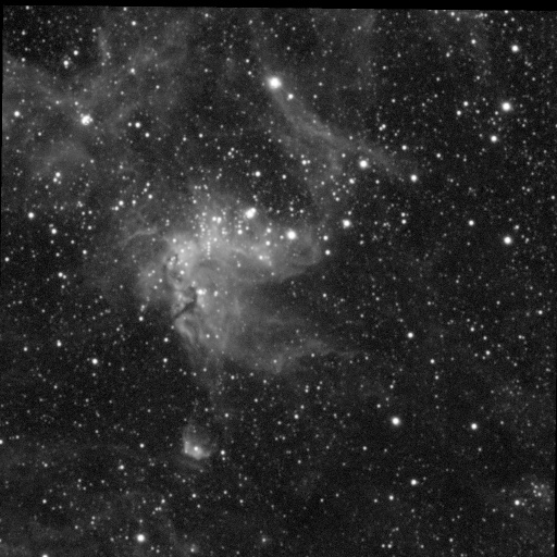
Figure 5— The red and H-alpha components plus the corresponding continuum map, with the same histogram adjustment applied.
Mouseover:
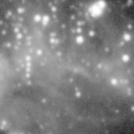
Figure 6— Same comparison as in Figure 5, on an enlarged crop. The continuum map shows many dim stars that were hidden by strong H-alpha nebulosity.
Mouseover:
As we have said before, to preserve the color balance of the stars and the depth of the narrowband image, commonly-used methods just mix both images. Our approach to this problem is much cleaner, as we do not mix both images, therefore we don't contaminate the high-quality narrowband image with noise from the broadband image. We are going to build a synthetic broadband image from the narrowband image. From the first equation, we can calculate the broadband image as:
B = N * C
Thus, by multiplying the narrowband image with the continuum map, we obtain the synthetic broadband image. Of course, as expressed above this operation would be useless, because we would just duplicate the original broadband image. What we need is emulating the intensities of all significant structures of the broadband image: we don't want to know the pixel-to-pixel intensity relation between both images, but the structure-to-structure relation. This is why we multiply the narrowband image by a continuum map to which we have applied a relatively strong noise reduction. In Figure 7 we show an example of this noise reduction.
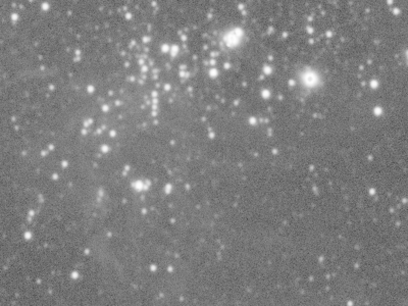
Figure 7— Comparison between the original and denoised continuum maps.
Mouseover: [Original continuum map] [Denoised continuum map]
As you can see, due to the poor signal to noise ratio of the R image in this example —remember that we intentionally added synthetic noise to simulate common acquisition conditions—, we were forced to apply a quite aggressive noise reduction to the continuum map. This had an adverse effect over the contrast of many dim stars. As a result, multiplying the H-alpha image by the denoised map didn't recover color balance completely for all of the stars in the image of this example. To overcome this problem, we apply the method iteratively: after multiplying the H-alpha image we obtain a second continuum map, then we apply a second noise reduction and make a second transformation to the image, and so on. Figure 8 shows the result of this iterative multiplication of the narrowband image by successive denoised continuum maps.
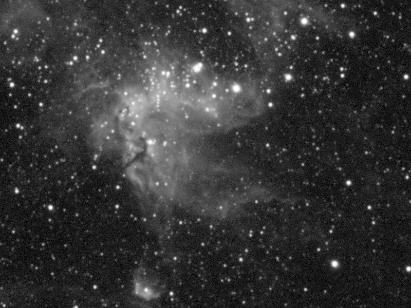
Figure 8— Iterative multiplication of the H-alpha image by denoised continuum maps.
Mouseover: [Original R image] [Original H-alpha image] [Synthetic R, 1 iteration] [Synthetic R, 2 iterations] [Synthetic R, 3 iterations]
As you can see on both figures, the synthetic red image represents the best of both imaging techniques: good colors on the stars and high signal-to-noise ratio in the nebulas. Some of the nebular structures have less contrast now, but don't worry because this will be overcome in the next section.
This synthetic red image will be used to create, along with the green and blue images, the RGB color composite. Pay special attention when comparing the resulting image to the original RGB image, on Figures 9 and 10. Finally, Figure 11 compares the results of our new HaRGB combination method, the maximum operator, and the channel-mixing combination method.
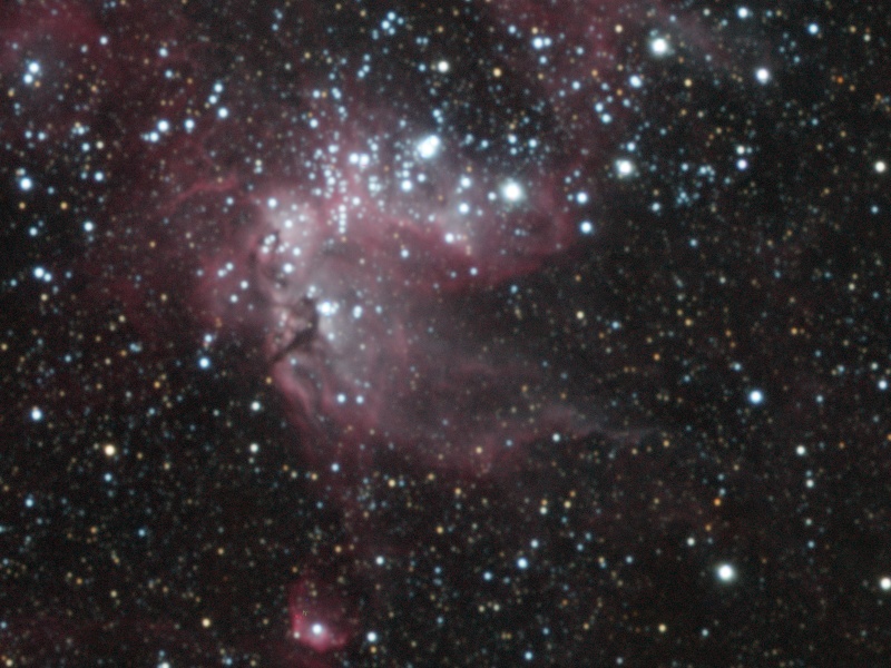
Figure 9— Original RGB image compared to the HaRGB image obtained with our method.
Mouseover: [Original RGB image] [Our HaRGB image]
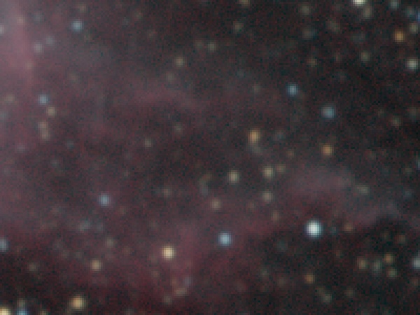
Figure 10— The same comparison as in Figure 9, on an enlarged crop.
Mouseover:
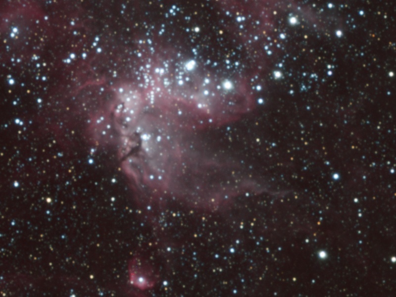
Figure 11— Our new HaRGB combination method compared to the maximum operator and the channel mixing method.
Mouseover: [HaRGB, our method] [HaRGB, maximum operator] [HaRGB, 50%/50% red and H-alpha blending]
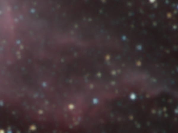
Figure 12— The same comparison as in Figure 11, on an enlarged crop.
Mouseover:
[HaRGB, 50%/50% red and H-alpha blending]
We have now a true HaRGB composite image, with no signal-to-noise ratio degradation, and with a correct overall color balance. Our first problem has been solved, so let's see how we'll solve the second one.
Again, the Dynamic Range Problem
We'll describe now the second part of our algorithm. Here we'll solve the star size problem, boosting the H-alpha signal, and recovering the contrast of nebular structures.
Perhaps one of the major problems that arise when combining narrowband and broadband images is the differing star sizes in both types of images. Narrowband imaging not only serves as a method to fight light pollution; it also unveils data that, in most cases, is lost under dense star fields. As a narrowband filter blocks all of the light except the light emitted by the object of interest (H-alpha emission in our working example), all of the stars in the image appear much fainter.
Let's take a look at the red and H-alpha images again, on Figure 13, after a midtones adjustment. Both images provide the same luminosities for equivalent light intensities: we have corrected them for the different exposures and background illumination levels. We can see them thanks to a nonlinear midtones transfer function.
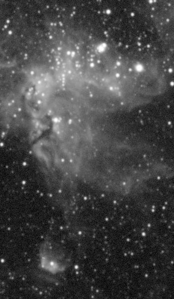
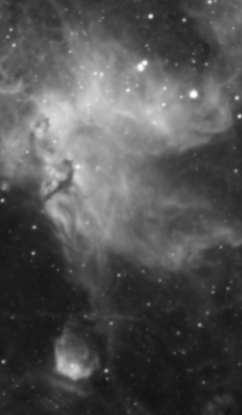
Figure 13— The red (left) and H-alpha (right) images, after applying the same nonlinear midtones transfer function.
Of course, the stars appear much larger in the broadband image (Figure 13, left). But let's compare the raw linear image on Figure 14: actually, star sizes are nearly the same on both (broadband and narrowband) linear images! So, which is exactly the real problem with stars, when combining narrowband and broadband data?
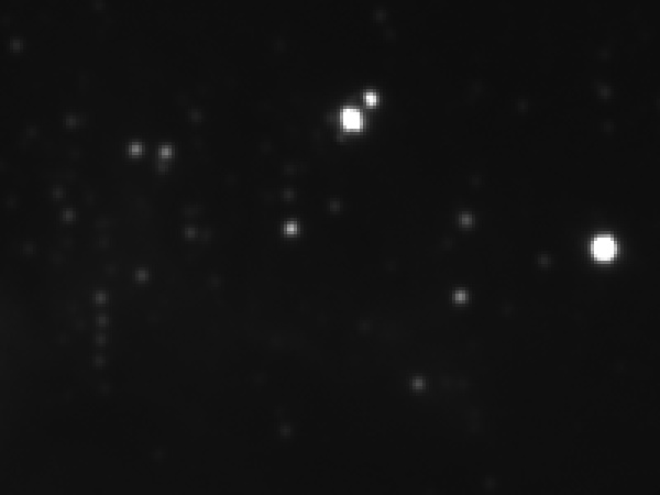
Figure 14— The linear (raw) red and H-alpha images. The main difference between stars in both images is not in their sizes, but in their brightness.
Mouseover:
As the title of this section suggests, the problem is, again, the dynamic range. In particular, the brightness ratio of stars to nebulas. Here is our real problem: if we simply combine the R and H-alpha images to make a color image, the result will be deeper for the nebulas, but all of those precious gradients of the nebula will be stolen in the resulting image due to the dominant star field.
One of the goals of this technique is, therefore, to emphasize emission line objects and at the same time, to diminish the protagonism of stars. Of course, this must be achieved without affecting the color balance of both types of objects. Keep this in mind: we are not going to decrease star size, but decrease star brightness.
Boosting H-Alpha Signal
Our method to enhance H-alpha objects in a color composite image is rather simple: we'll make a second color image, but this time the red channel will be the pure H-alpha image. We'll multiply the H-alpha image by a given factor, as illustrated in figure 15.
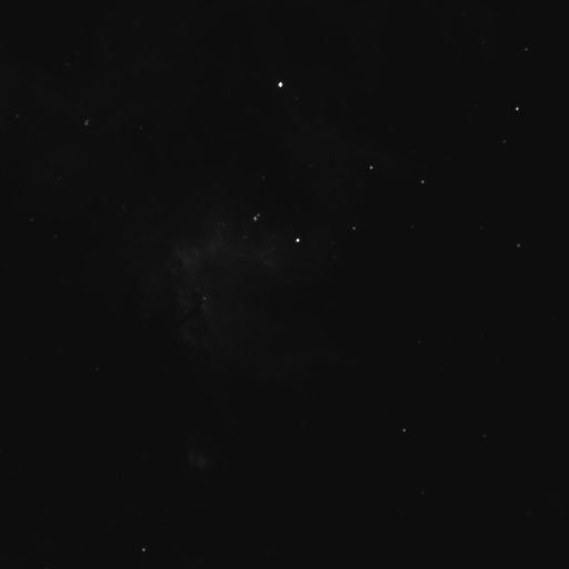
Figure 15— The linear H-alpha image, multiplied by several constants.
Mouseover:
[×1]
[×2]
[×4]
[×8]
Then we'll make a RGB composite with this new image. For this example, we'll use a multiplying factor of 12, as seen on Figure 16. Now if we apply a histogram adjustment, the image becomes extremely red, as expected.
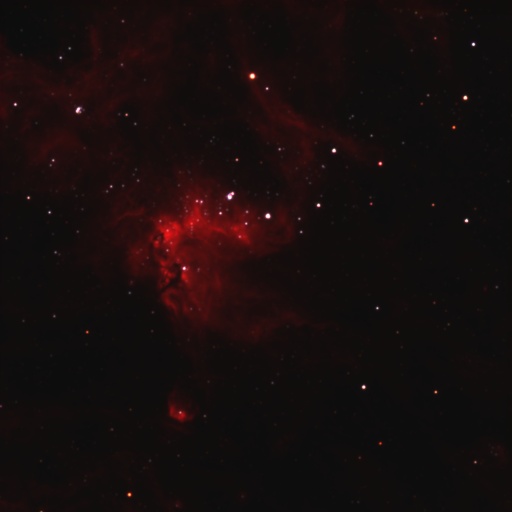
Figure 16— The Ha(x12)GB linear image, before and after a midtones transfer function.
Mouseover:
[HaGB composite with a midtones transfer function of 0.015]
Don't panic, because we are going to correct this image with our wonderfully deep and noise-free chrominance. A precondition to obtain a good chrominance transference between two images is to have a good correspondence between their luminances. In first place, we must apply the same histogram adjustment to the HaRGB and HaGB images. Second, we'll assign a linear RGB working space (RGBWS) to both images. A linear RGBWS has a gamma value of 1.0. In a linear RGBWS, we obtain much flatter luminances, as can be verified in Figures 17 and 18.
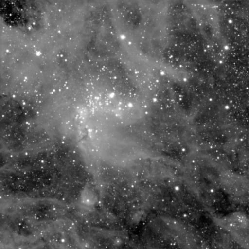
Figure 17— The luminance of the HaGB image in different RGB working spaces.
Mouseover:
[HaGB composite luminance, gamma = 2.2]
[HaGB composite luminance, gamma = 1.0 (linear RGBWS)]
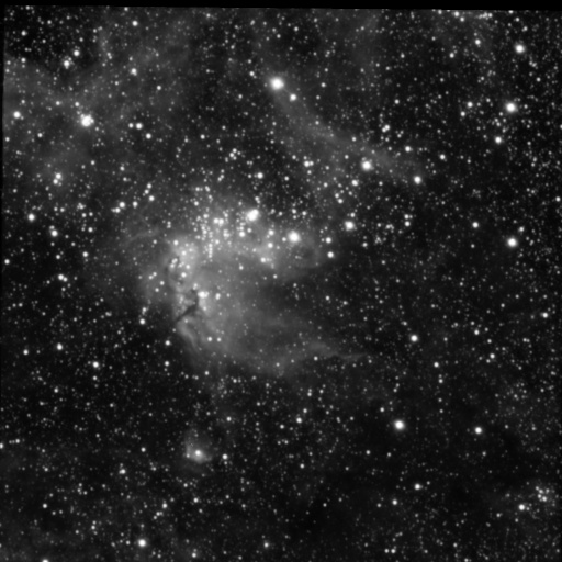
Figure 18— The luminance of the HaRGB image in different RGB working spaces. Note that with gamma = 2.2, there is a significant difference between the HaRGB luminance and the HaGB luminance (see Figure 17). However, with gamma = 1.0 both luminances are very similar.
Mouseover:
[HaRGB composite luminance, gamma = 2.2]
[HaRGB composite luminance, gamma = 1.0 (linear RGBWS)]
Once we have the best fit between both luminances, we'll transfer the CIE a* and CIE b* components from the HaRGB composite to the HaGB composite. The resulting color-corrected image can be seen on Figure 19.
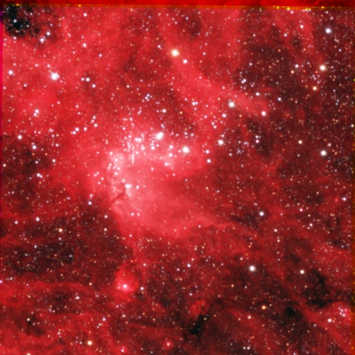
Figure 19— Chrominance correction. The CIE a* and b* components (in the CIE L*a*b* space) have been transferred from the HaRGB image to the HaGB composite.
Mouseover:
Finally, to better illustrate the H-alpha boosting effect, let's analyze the sequence shown in Figure 20. As you probably have noted, larger H-alpha boosts cause some loss of contrast in the highlights. Correcting this adverse effect is very easy with the High Dynamic Range Wavelet Transform algorithm, which has been implemented as the HDRWaveletTransform tool in PixInsight. Figure 20 shows the results of several boosting factors applied with some easy processing steps: HDR wavelets, RGB and color saturation curves adjustments.
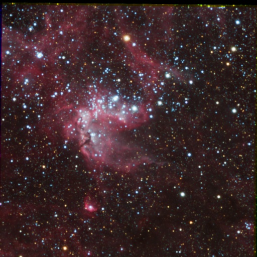
Figure 20— The final HaGB composite image with different H-alpha boosting factors.
Mouseover: