Dynamic Range and Local Contrast
Tutorial by Vicent Peris (PTeam/OAUV/CAHA)
Introduction
In this tutorial I describe some techniques I've been using on my latest images. The main goal of these techniques is to control the dynamic range and local contrast of an image of NGC 7023 (Iris nebula) acquired with the 1.23 meter Zeiss telescope at Calar Alto Observatory, in Southern Spain. This image is part of the Descubre/CAHA/OAUV/DSA collaboration. Data acquisition and processing have been carried out by Jack Harvey (SSRO), Steven Mazlin (SSRO) and Vicent Peris (OAUV).

NGC 7023 image processed with the techniques described in this tutorial.
Click on the image to see a full-size version.
Controlling the dynamic range of an image means to equalize the contrast of all the structures throughout all the dimensional scales. When this is achieved, no structure shows an excess of contrast compared to the rest of structures in the image. To implement this task, we are going to use mainly four PixInsight tools: HDRWaveletTransform, LocalHistogramEqualization, GradientsHDRCompression, and the MaskedStretch script.
First Dynamic Range Compression
We start with an already stretched (nonlinear) image. The midtones of the image have been adjusted to make the details in the darker clouds well visible. As can be seen on the image in Figure 1, this enhancement of the midtones has left the center of the nebula almost saturated.
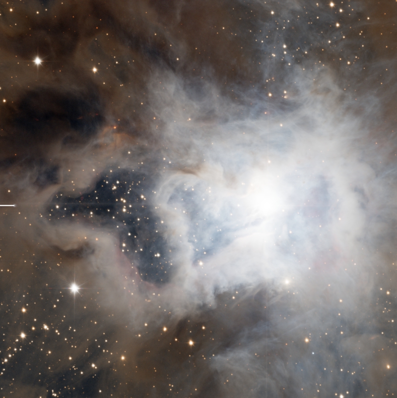
Figure 1— Stretched image of NGC 7023.
The first step is obvious: to compress the dynamic range of the image with the HDRWaveletTransform tool (HDRWT). As we have a lot of fine detail, we use only five wavelet layers. We activate the luminance mask option to restrict application of the HDRWT algorithm to the most illuminated areas. The result can be seen in Figure 2.
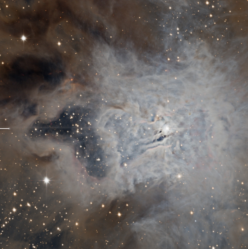
Figure 2— Initial dynamic range compression with HDRWaveletTransform applied to the image on Figure 1.
High-Contrast, Small-Scale Structures
One problem inherent to all techniques employing kernel filters as scaling functions is that they cannot model high-contrast structures at very small dimensional scales. As a result of this limitation, the dynamic range of these structures remains uncompressed. This problem becomes evident for the stars, as you can see on Figure 3.
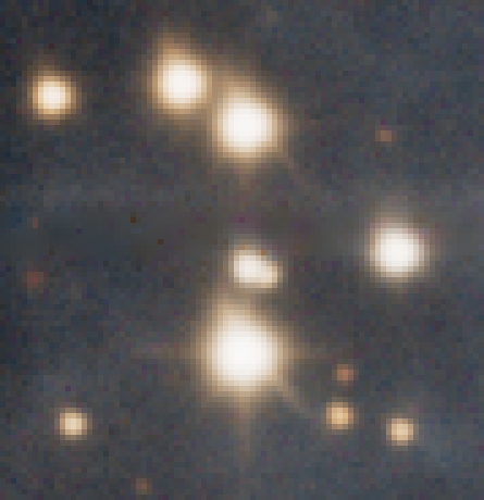
Figure 3— The stars are almost saturated with hard edges after HDRWaveletTransform.
The MaskedStretch script has been written by David Serrano, with contributions from Andrés del Pozo, based on an original algorithm designed by Carlos Sonnenstein. The algorithm performs successive masked histogram transformations until it reaches a prescribed average background value, which can be specified as the target median parameter. The applied masks are generated dynamically at each iteration. One of the advantages of this algorithm is that it doesn't rely on any scaling function. As a result, it does an extremely good job at compressing the dynamic range of the high-contrast, small-scale structures that can't be modeled with multiscale techniques.
For the NGC 7023 image, we run the MaskedStretch script (MS) on the linear (unstretched) image and set its target median parameter to the median value of the stretched image after HDRWT (0.43 in this case). In this way we can achieve similar brightness and contrast for the whole image with both techniques. It is important to point out that we don't select any mask blurring method on the MS script, as that would alter the stars on the mask and hence would reduce the effectiveness of this technique for dynamic range compression. The applied settings can be seen on Figure 4, and the resulting image on figures 5 and 6.
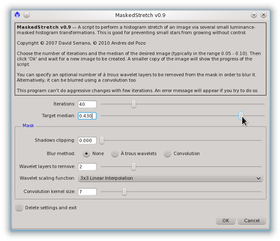
Figure 4— The MaskedStretch script interface with the parameters selected for this example. In this case we apply 40 iterations. The target median of 0.43 is the same value obtained for the image previously stretched and processed with HDRWT (see Figure 2).
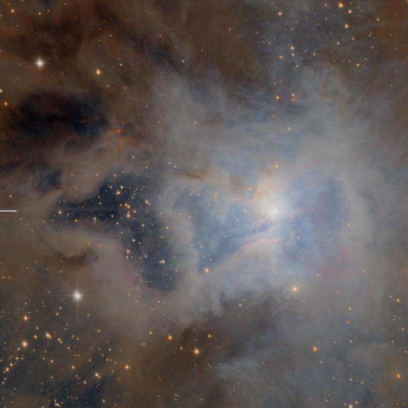
Figure 5— The resulting image after applying the MaskedStretch script with the parameters shown on Figure 4.
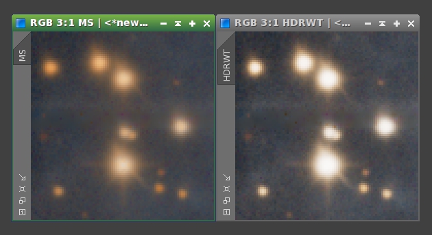
Figure 6— The same crop taken from the images on Figure 5 (left) and Figure 2 (right). The stars are much softer and less saturated after MaskedStretch (left) than they are after applying HDRWaveletTransform to a stretched image (right).
The overall small-scale contrast of the image processed with the MaskedStretch algorithm is very low, as evidenced by Figure 5. We only want to use this result on the regions that actually can benefit from it: Those regions where HDRWT does not work properly. So if we use a mask to combine the MaskedStretch result with the nonlinear image after HDRWT, we can get the best of both techniques.
To build this combining mask we need to know the answer to the following question: Where are the largest differences between the HDRWT and MaskedStretch processed images? In other words, we are going to calculate the difference between both images, so the mask will protect the areas where both images are similar. This can be done with the PixelMath tool. We operate with the lightness components (CIE L*) of both images. The result of MaskedStretch will be subtracted from the HDRWT image. The resulting mask can be seen on figures 7 and 8.
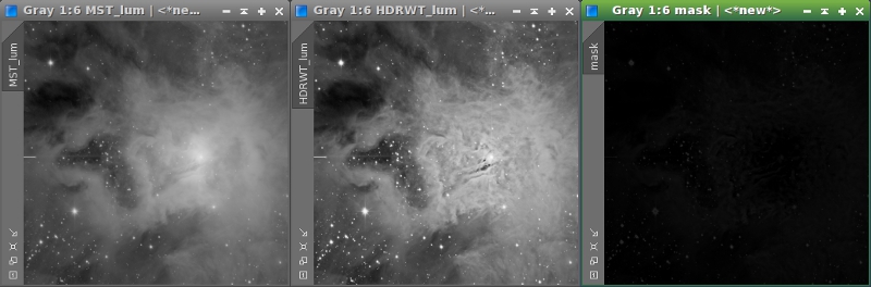
Figure 7— The lightness components of the MaskedStretch result (left) and the HDRWT image (middle), and the result of subtracting the former from the latter (right).
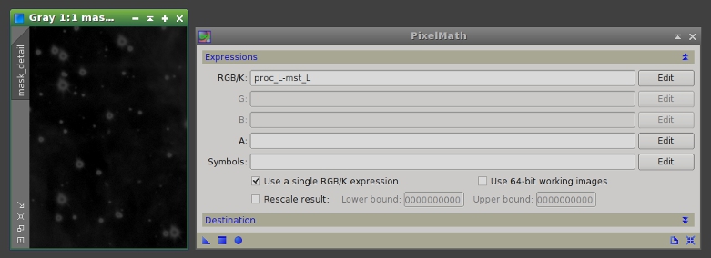
Figure 8— To the left, a detailed view of the combining mask. Note that this mask selects the star edges. To the right, the applied PixelMath parameters. The rescale result option of PixelMath has been disabled because we are only interested in positive differences, which represent all of the bright and small structures. The output is sent to a new image whose identifier will be "starmask".
This mask also selects a lot of structures on the core of the nebula. Combining the images in this way would lead to a loss of contrast in these structures. To prevent this problem we are going to modify the mask. As we are interested only in small structures, the large-scale structures can be erased very easily with the ATrousWaveletTransform tool by disabling the residual (R) layer (Figure 9).
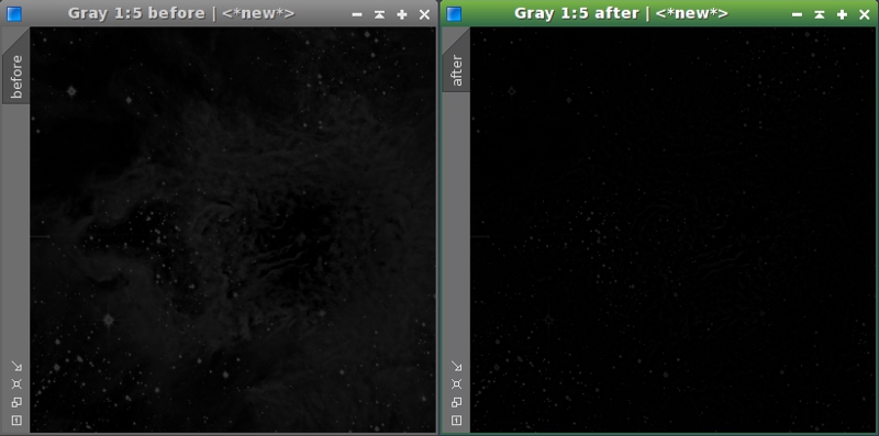
Figure 9— The separation between the stars and all the nebula structures can be enhanced by leaving only the first wavelet layers. To the right, the result of removing the residual layer with the ATrousWaveletTransform tool.
The final mask adjustments are done with the MorphologicalTransformation and ATrousWaveletTransform tools. We first apply a dilation filter in order to extend the mask to cover the external areas of the stars. Finally, we smooth the mask a little bit by removing the first wavelet layer. These processes are described on figures 10 and 11.
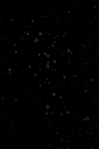
Figure 10— Final mask adjustments.
Mouse over:
10a— Original mask.
10b— After applying a dilation filter.
10c— After removing the fist wavelet layer.
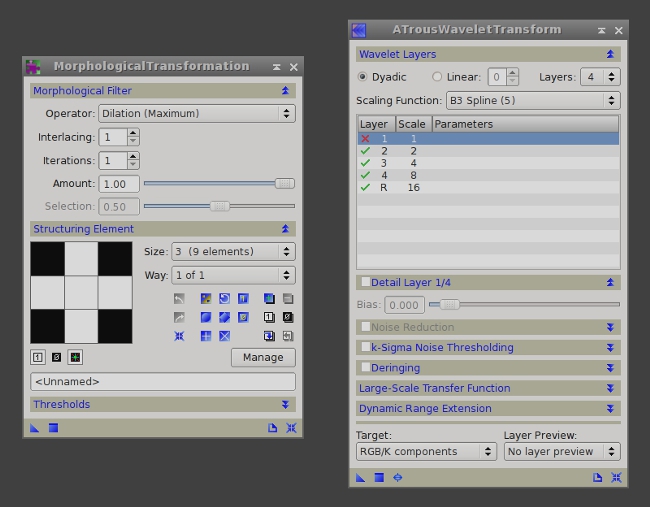
Figure 11— Instances of MorphologicalTransformation and ATrousWaveletTransform with the applied parameters.
Once we have finished the mask, we are going to use it to fix the stars. This process consists of transferring the small scales of the image processed with MaskedStretch to the HDRWT processed image. First we create working duplicates of both images. Since these duplicates will only have the medium- and large-scale structures, we'll assign the MS_LS and HDRWT_LS identifiers for clarity. Now we remove the first five wavelet layers of MS_LS and HDRWT_LS (Figure 12). This procedure results in the four images that you can see on Figure 13.
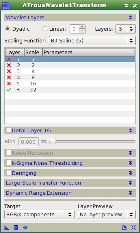
Figure 12— ATrousWaveletTransform instance used to remove the first five wavelet layers from the working duplicate images.
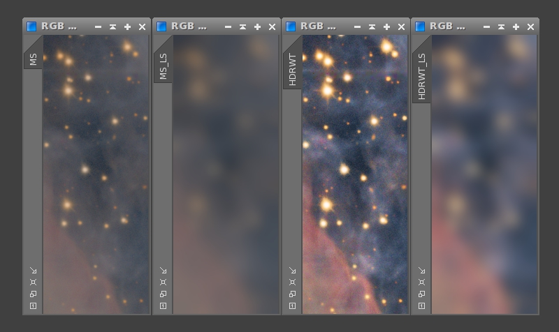
Figure 13— A comparison of the four images on a full-size crop: the two originally processed images, MS and HDRTW, and their low-pass filtered versions MS_LS and HDRWT_LS, respectively.
To transfer the small scales of the image processed with MaskedStretch (MS) to the HDRWT image, we use the following PixelMath expression (Figure 14):
MS - MS_LS + HDRWT_LS
Speaking in multiscale terms, the above expression replaces the large-scale components in the MS image with the corresponding components of the HDRWT image. This process must be masked with the mask we have built in the preceding paragraphs. This mask has very low pixel values (0.1 to 0.2 on the star edges), so we can apply the same PixelMath instance iteratively to control the intensity of the process. This allows us to adjust the desired amount of dynamic range compression on these small-scale structures. In Figure 15 we can see how the stars recover their natural Gaussian profiles throughout successive PixelMath iterations.
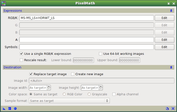
Figure 14— The PixelMath instance used to transfer structures from the MS image to the HDRWT image.
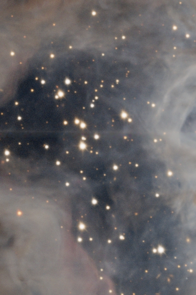
Figure 15— By applying several iterations of the same PixelMath instance (see Figure 14) we can gain tighter control over stellar profiles.
Mouse over:
15a— Original HDRWT image.
15b— One PixelMath iteration.
15c— After two iterations.
15d— After three iterations.
15e— After four iterations.
15f— After five iterations.
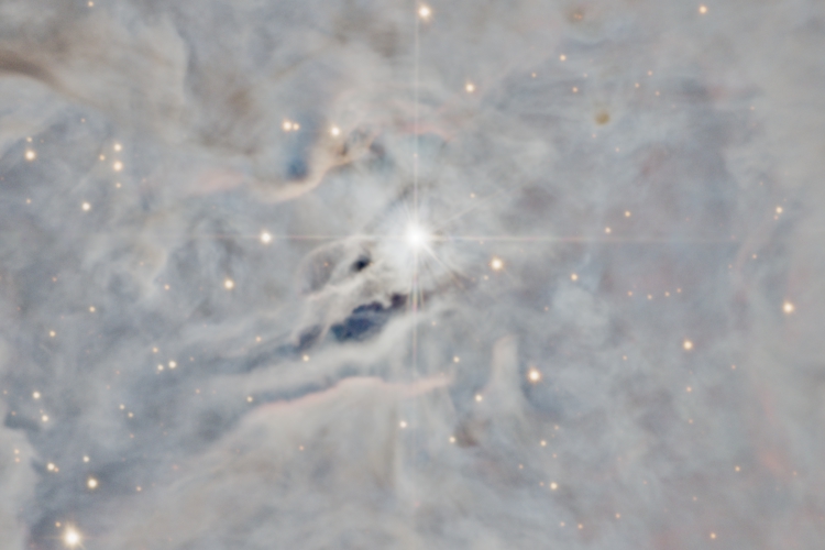
Figure 16— A comparison of the image before and after transferring small-scale structures, on a full-size crop near the center of the main nebula.
Mouse over:
16a— Original HDRWT image.
16b— After five PixelMath iterations.
Local Enhancement
After applying the HDRWT algorithm the structures in the core of the nebula have been recovered, but this area still has a very low local contrast. When this happens, the LocalHistogramEqualization tool does a very good job. LocalHistogramEqualization is an implementation of the Contrast Limited Adaptive Histogram Equalization algorithm (CLAHE), written by Czech software developer and PixInsight user Zbynek Vrastil.
Before applying LocalHistogramEqualization (LHE), we need to protect the stars to preserve their shapes. We are going to mask the LHE process through a modified version of the star mask we created in the preceding section. To modify the mask we use the MorphologicalTransformation, ATrousWaveletTransform, HistogramsTransformation and CurvesTransformation tools. This is well exemplified in Figure 17.
Figure 17— Steps to build the local enhancement mask.
Mouse over:
17a— Original mask.
17b— Histogram transformation.
17c— First morphological transformation.
17d— First smoothing with ATWT.
17e— Second morphological transformation.
17f— Second smoothing with ATWT.
17g— Curves transformation.
Once we have adjusted the mask we can apply LHE to the image. We load the mask and invert it, so the stars remain protected. In the LHE process, we have used the default kernel radius and amount parameters. The contrast limit parameter has been set to 1.7.
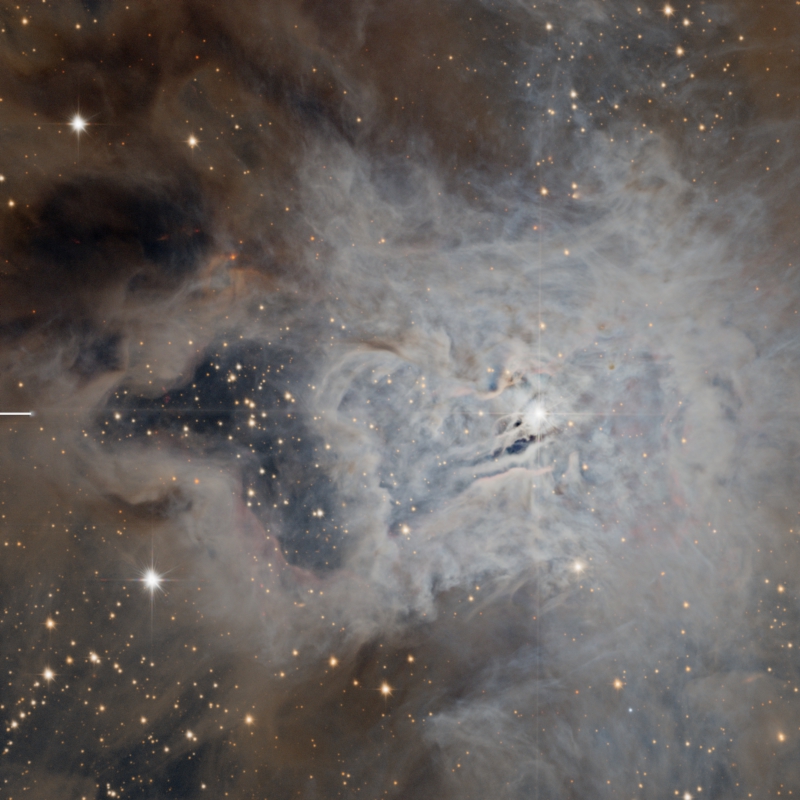
Figure 18— Although the structures in the core of the nebula have been recovered by the HDRWaveletTransform algorithm, The LocalHistogramEqualization tool is very useful to equalize the local contrast of the whole image.
Mouse over:
18a— Before LocalHistogramEqualization.
18b— After LocalHistogramEqualization.
Another problem arises now: lack of color saturation. This is a downside of the techniques that enhance the image locally, as they decrease the color saturation at larger scales in favor of enhancing hues at smaller scales. This can be corrected easily with a simple curve applied to the S component with the CurvesTransformation tool (see figures 19 and 20).
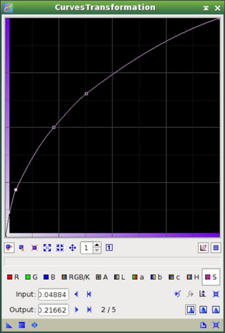
Figure 19— The curve applied to the S component in order to raise the color saturation of the image. The result can be seen on Figure 20.
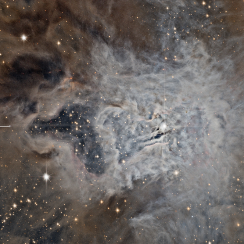
Figure 20— The effect of raising the color saturation with CurvesTransformation (see Figure 19).
Mouse over:
20a— Before color saturation enhancement.
20b— After color saturation enhancement.
Finally, at this stage it is always very useful to apply an S-shaped curve to the combined RGB/K channel with CurvesTransformation. This enhances contrast on the brightest areas. We apply the curve through a luminance mask, as described in figures 21, 22 and 23.
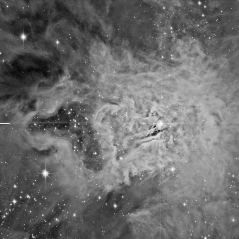
Figure 21— We extract the lightness component (CIE L*) of the image and select it as a mask before applying CurvesTransformation.
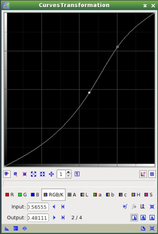
Figure 22— The curve applied to the brightest areas of the image, masked with the lightness component shown on Figure 21. The result can be seen on Figure 23.
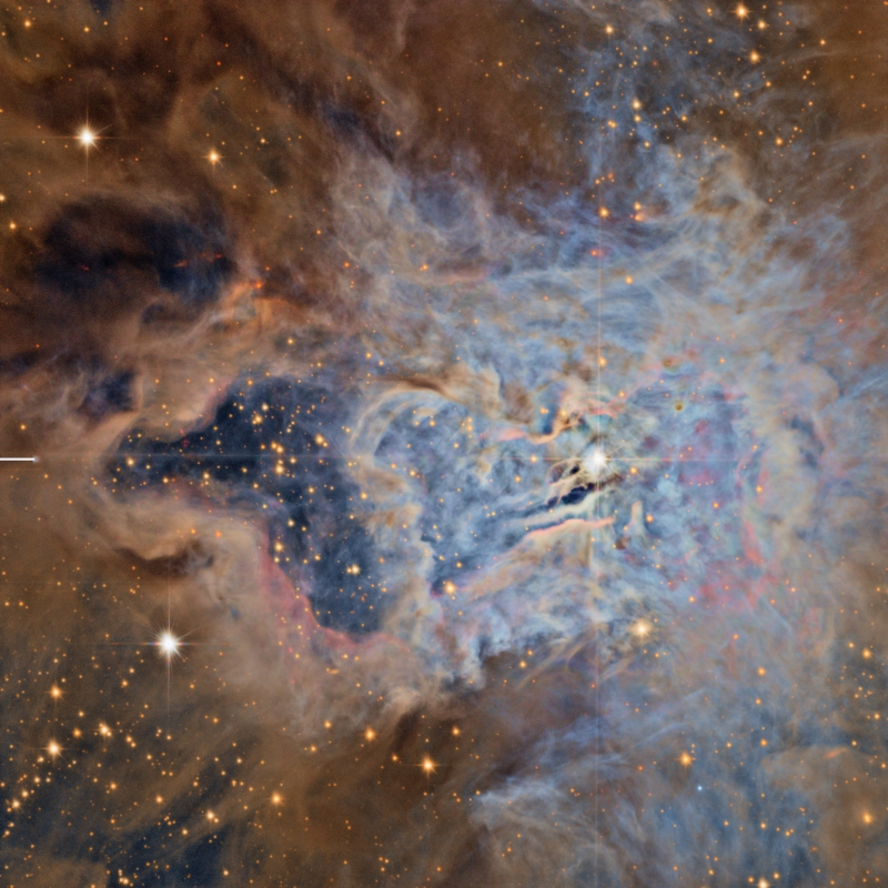
Figure 23— The effect of applying an S-shaped curve to the combined RGB/K channel through a luminance mask (see figures 21 and 22).
Mouse over:
23a— Before CurvesTransformation.
23b— After CurvesTransformation.
Deringing
Both HDRWaveletTransform and LocalHistogramEqualization can generate ringing artifacts around very high contrast structures at medium and large dimensional scales. This is clearly shown for the image of this tutorial in the dark lanes around the central star, on Figure 24.

Figure 24— On this full-size crop, the dark structures have been over darkened because their local contrast is very high.
Although HDRWT has its own deringing parameters, we are going to fix these ringing artifacts manually. One way to correct these artifacts is with PixelMath. To know how much ringing has the image we can calculate the ratio of the pixel values between the original image and the one processed with HDRWT and LHE. In Figure 25 we can see the applied PixelMath instance.
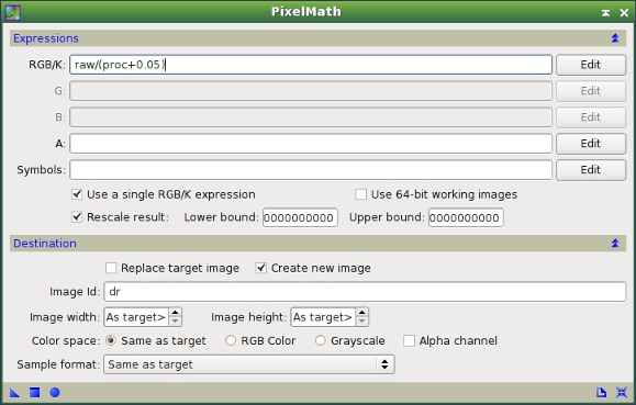
Figure 25— PixelMath instance to calculate the variation of pixel values between the original and the processed images. "raw" is the linear image, just before the initial histogram transformation; "proc" is the image processed with HDRWT, LHE and CurvesTransformation, as described above.
As shown on Figure 25, we use the PixelMath expression:
raw/(proc + 0.05)
to calculate the ratio between the linear (raw) and processed (proc) images for each pixel. We add a small pedestal of 0.05 in order to prevent divisions by values very close to zero. The Rescale result option is enabled and we send the output to a new image with the "dr" identifier. The result is a ringing map, that is an image showing where ringing artifacts occur, which you can see on figures 26 and 27.
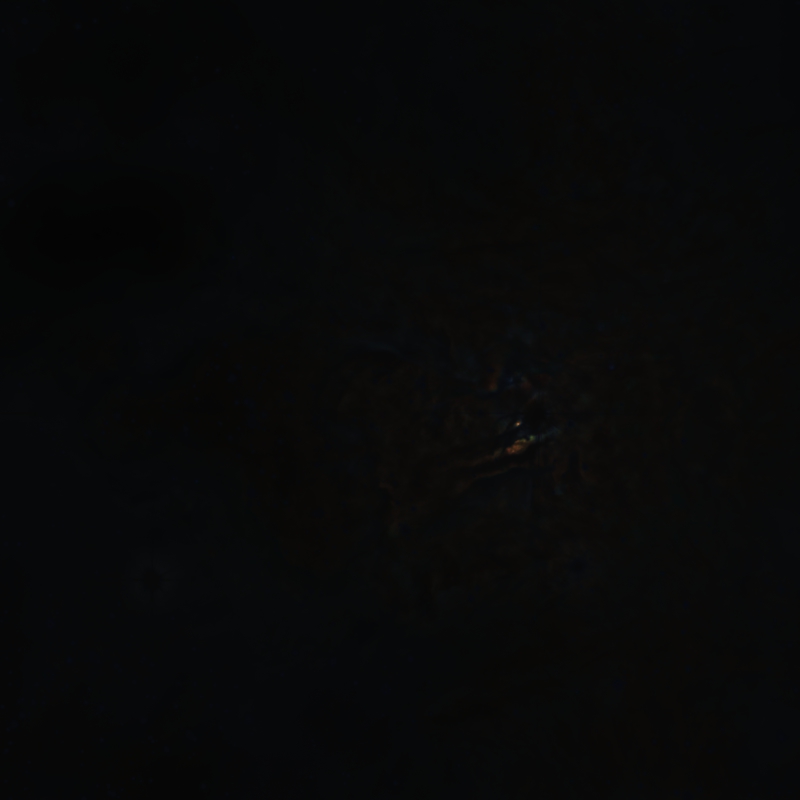
Figure 26— The ringing map clearly shows the problematic areas as bright structures. These are mainly adjacent areas to the central star. This happens because the pixel values of these structures have been lowered during the applied processing, reaching values close to zero. Therefore, the division applied to the original image (see Figure 25 and the comments above) produces very high values on these areas.
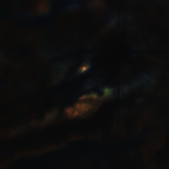
Figure 27— A full-size crop of the ringing map shown on figure 26, centered on the dark structures where ringing mainly occurs.
Before applying the ringing map to the image we can improve its efficiency by increasing the isolation between the problematic structures and the rest of structures in the image. This can be easily done with CurvesTransformation, as shown on Figure 28.
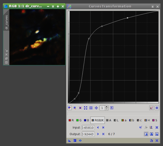
Figure 28— Curve used to enhance the ringing map. In order to increase contrast of bright ringing map structures while keeping the other map structures almost black, this curve has to be very steep between its initial and final sections. To build this kind of curves the Akima subspline curve interpolation (enabled by default in CurvesTransformation) is very useful.
Now we can correct these structures with PixelMath. We add the modified ringing map, multiplied by a scaling factor (0.15 in this case), to the already processed image. See figures 29 and 30.
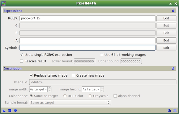
Figure 29— PixelMath instance to add the (scaled) ringing map to the processed image.
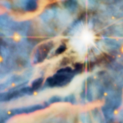
Figure 30— The effect of ringing correction.
Mouse over:
30a— Before ringing correction.
30b— After ringing correction.
The result, as shown on Figure 30, still has very dark structures, but this will be further corrected in the next section of this article.
Gradient Domain Operations
To conclude the dynamic range related processing techniques, the last step is carried out by operating in the gradient domain. This step will decrease the contrast of some structures around the center of the nebula. It will also help in fixing the remaining ringing artifacts completely. These structures are still problematic because they have too much contrast in comparison with the rest of the visual information in the image. In this section we are going to use the GradientsHDRCompression tool (GHC), written by Georg Viehoever. Gradient operations, when used for dynamic range compression, use to be tricky and should be applied with caution. One drawback is that they tend to generate opaque stars. This problem can be seen on Figure 31.
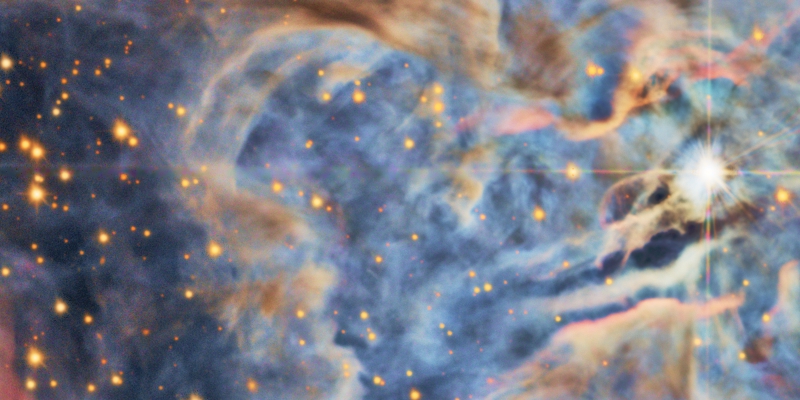
Figure 31— GHC tends to opacify the stars whose central values are sensibly below unity. This effect is clearly shown on the stars at the left side of this full-size crop.
Mouse over:
31a— Before GradientsHDRCompression.
31b— After GradientsHDRCompression.
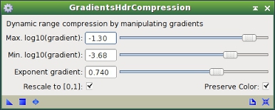
Figure 32— GradientsHDRCompression instance. The exponent gradient parameter allows us to control the contrast of dark structures. Oppositely, the Max.log10(gradient) parameter provides control over the contrast of bright structures. Adjust the latter parameter with great care; it is very sensitive.
Consequently, this process must be applied with the protection of a star mask. We are going to use the same modified star mask we applied before, again inverted in order to protect the stars.
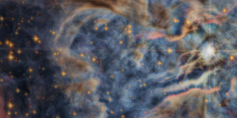
Figure 33— By applying the GradientsHDRCompression process through an inverted star mask we can protect the stars and avoid the problems shown on Figure 31.
Mouse over:
33a— GradientsHDRCompression applied unmasked.
33b— GradientsHDRCompression applied with an inverted star mask.
Now if we look at the entire image, we can see that it has been darkened globally. We are going to raise a bit the midtones of the image with HistogramTransformation, but we have to apply this again through the inverted star mask in order to modify only the processed areas of the image.
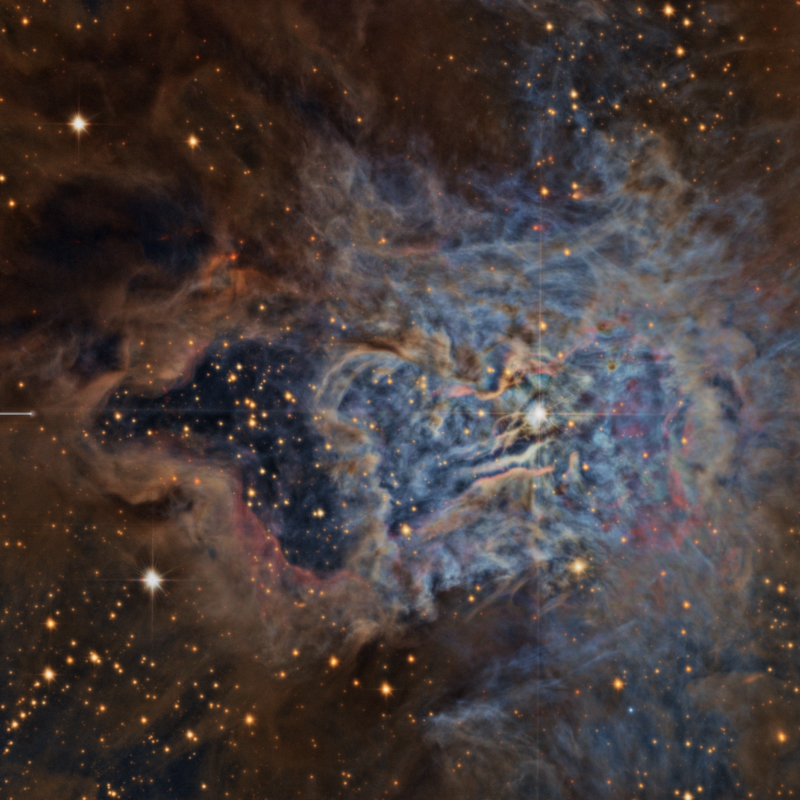
Figure 34— The effect of raising the midtones with HistogramTransformation after GradientsHDRCompression. A midtones balance value of 0.38 has been used.
Mouse over:
34a— Before HistogramTransformation.
34b— After HistogramTransformation.
Figure 35— A comparison on a full-size crop near the center of the nebula.
Mouse over:
35a— Before GradientsHDRCompression.
35b— After GradientsHDRCompression + HistogramTransformation.
Final Processing Steps
After applying dynamic range processing techniques —especially when we apply those techniques that affect small-scale structures— we usually need to recover the sharpness of the image. This can be done with the ATrousWaveletTransform tool, by applying positive biases to the 1- an 2-pixel scales. Here we also need a lightness mask to protect the image from excessive noise intensification on the lower signal-to-noise ratio areas.
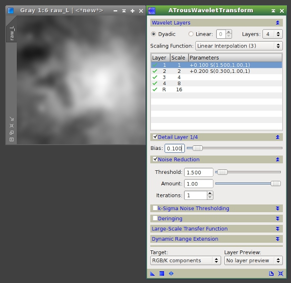
Figure 36— The lightness mask and the ATrousWaveletTransform instance used for sharpening. Noise reduction has also been enabled for the two modified wavelet layers.
Figure 37— The effect of recovering the sharpness of the image with wavelets. Note that, thanks to the applied dynamic range compression techniques, the sharpening process can be implemented with much tighter control because the image does not have structures with excessive contrast.
Mouse over:
37a— Before sharpening with ATrousWaveletTransform.
37b— After sharpening with ATrousWaveletTransform.
Final Thoughts
PixInsight has a flexible toolset for controlling the dynamic range of your images. Usually the HDRWaveletTransform tool gives very good results for this task. However, to achieve a superior result we need to go beyond this tool. In this article we have used several tools, putting into practice very different approaches to the same problem. The key of these procedures is to apply each tool when and where it is needed.
It is equally important to understand that the application of these techniques will ease most subsequent processing steps. From a sharpening process to a simple curve, all of these processes will be more powerful and efficient if the contrast of our image has been previously diminished at a wide range of dimensional scales.