ManualImageSolver

2.1 Reference image

ManualImageSolver requires a reference image that covers completely the target image. This image should be of good quality, it must have enough stars in the entire area of the target image and it must have a high quality coordinates solution. Although a real image can be used, the best results are achieved using a synthetic image generated using CatalogStarGenerator. CatalogStarGenerator can easily generate a good quality image of any part of the sky.

These are a few suggestions for generating the reference image:

• Use a resolution (or focal length) not too different to the target image. A factor of 2 should be good enough. i.e. if the target image has an estimated resolution of 2 sec/pix, the reference image should have a resolution between 1 and 4.
• The reference image must contain the entire target image. It doesn't mind that the reference image is bigger than the target, but the reference must cover the entire target.
• Chose a suitable projection for the image. For most images the Gnomonic projection is the best one. For very short focal length images (i.e. all-sky cameras, fisheye lenses) Orthographic or Zenithal Equal Area could be better.
• For wide field images the best catalog in CatalogStarGenerator is "BrightStars". This catalog contains most stars with magnitude up to 7.
• For higher resolution images the catalog PPMXL can be used, although it is necessary to filter the maximum magnitude to adapt it to the magnitude of the image. It is important to know that PPMXL shouldn't be used for wide field images because it doesn't contain some bright stars and the downloads are very slow for big areas.
• The script AnnotateImage can be used for drawing lines or labels that simplify the recognition of the stars in the synthetic image. For example, for wide field images is useful to draw the constellation lines on the reference image. This should be done so that the markings don't interfere with the star detection of DynamicAlignment: you can not set a control point on a star if it is covered by a label or line.

2.2 Control points

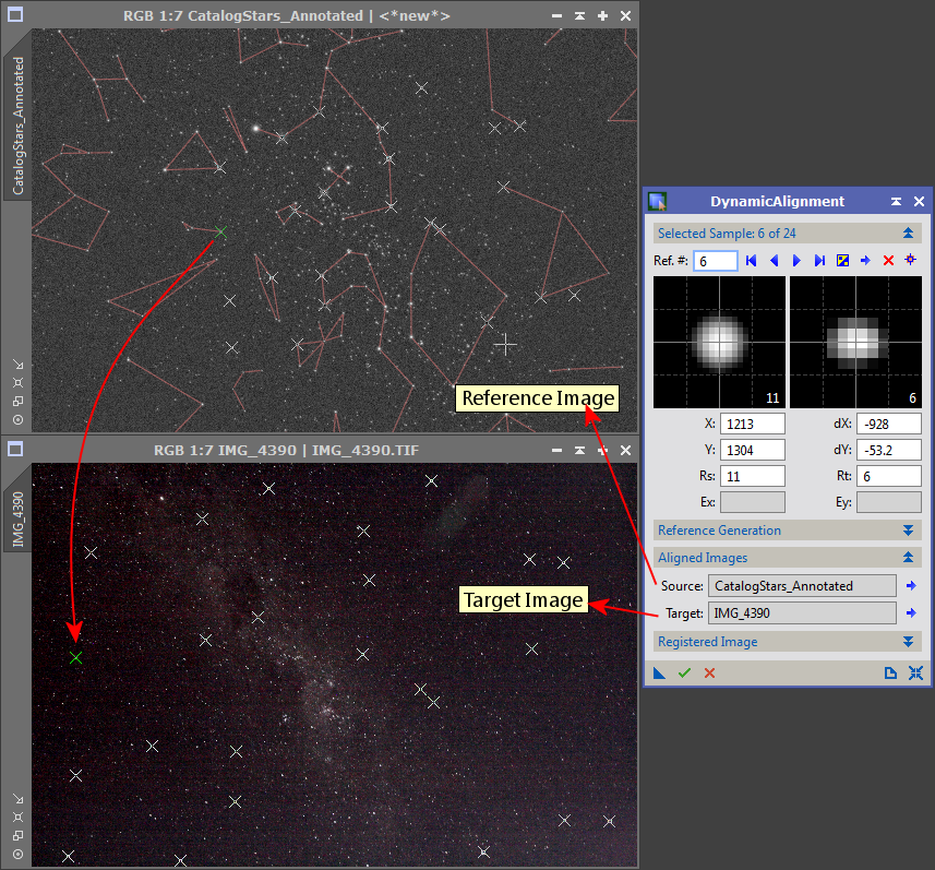
The control points are pairs of points in the reference and target images that correspond to the same coordinates, usually the same star. The control points can be defined using the process DynamicAlignment. After opening the reference and target images in PixInsight you have to launch the process DynamicAlignment. The reference image must be selected as "Source" (first) and the target image as the "Target" (second). The process of selecting the control points is this:

• Identify the same star in both images.
• Click in the position of the star in the reference image.
• Find the position of the new control point in the target image and move it to the position of the star.

Identifying the same star in both images is perhaps the hardest part of the process. Fortunately, after two or three control points have been set DynamicAlignment can predict the approximate position of the control points in the target image. Because of this, only the two first points are really difficult to match in both images. After them, the rest of points can be matched using the prediction of DynamicAlignment and some common sense.

After selecting enough control points you have to save the DynamicAlignment process to a process icon. This is done dragging the triangle at the lower left corner of the interface window to the workspace.

These are a few suggestions for selecting the control points:

• You should select control points covering the entire image. There should be control points near the corners of the image.
• The quality of the solution depends on the number of control points and their quality. The necessary number of control points depends on the strength of the distortion of the image: An image with no distortion can be solved with only three control points although it is better to use more control points. An image with strong distortions can require 40 or more control points.
• If the image has much noise it is advisable to select more control points.
• After selecting the first two control points, DynamicAlignment tries to predict the position of the control point in the target image. Sometimes this prediction fails and it selects a wrong position. You have to be aware of this, check every control point and move them to the correct position when necessary.
• The script can not detect if any of the control points has a wrong position (i.e. a star misidentified in one of the images). This case can be detected analyzing the residuals image that the script can optionally generate (see Generate residuals image). If a control point is wrong, its residuals (red line in the residuals image) will be much greater than the residuals of the rest of the points. After identifying the misplaced control point, you can fix (or delete) it and rerun the script.

2.3 Execution of ManualImageSolver

As the final step you have to run the script ManualImageSolver. This script analyzes the control points and the reference image and calculates a solution for the coordinates of the target window.

ManualImageSolver works on the active window in PixInsight. When you run the script it shows its configuration dialog:

Control points icon

This parameter shows a list of the DynamicAlignment icons available in the workspace. You have to select the icon that contains the control points that you want to use for solving the image. This icon can be created using the process explained in the section Control points.

Reference image

This parameter shows a list of all the images open in PixInsight that have coordinates defined. You should select the image that was used for creating the control points icon or one with exactly the same geometry and coordinates.

Generate residuals image

When this option is selected the script generates an image which shows the residuals of the solution. The image shows as green crosses the predicted position of the control points using the calculated solution. Red lines from each control point join the predicted position to the actual position marked by the user.

This image can be used to analyze the errors of the solution. In a good solution all the red lines should be very short (in a perfect solution the lines should have degenerated to points). When there is a control point with misplaced position its red arrow is much longer than the rest of control points.

Distortion correction

This parameter activates the distortion correction using surface splines. This option should be selected when the image deviates from an ideal projected image. This usually happens in images taken with focal lengths shorter than 400mm.

When this option is active the script stores the solution in the properties of the image using a non-standard format. In order to be able to use the solution in other applications, the script also computes a lineal solution (without distortion correction) and stores it in the keywords of the image in the WCS format.

The options Show distortion map and Generate residuals image can help to evaluate the quality of the distortion correction.

Show distortion map

When this option is activated the script creates a new window with a representation of the distortions in the image. The new image contains a grid with arrows at the center of each cell. The arrows point to the point where the center of the cells would be located if the image didn't have optical aberrations.

This option is only enabled when the distortion correction is active.

Figure 1

Generate distortion model

The script generates a CSV archive with a distortion model that consists in a list of points and their displacement relative to an ideal image with no geometrical optical aberrations. The points used in the model are the control points, so the control points should cover the whole image for best results. The distortion model is compatible with StarAlignment and ImageSolver.

This option is only enabled when the distortion correction is active.

When the script finishes successfully, stores the coordinates in the image and the console shows the values of this solution.

The quality of the solution can be checked analyzing the value of the RMS error reported in the console, analyzing the residuals image and using AnnotationScript for drawing a grid and the position of the stars on the target image.

3.1 Solution optimization

Since the process of defining the control points for ManualImageSolver is quite slow and tedious, the user usually will not want to define more than 30-40 control points. Although this number is enough for calculating a good solution for most images, the quality of the solution is not comparable to the solutions calculated by ImageSolver which can use several hundreds of samples.

The solutions calculated by ManualImageSolver can be optimized using ImageSolver. Although ImageSolver can not solve some images starting from scratch, when these images are already solved, ImageSolver can be used for further improving the solution.

After solving the image using ManualImageSolver you can run ImageSolver selecting the option "Only apply optimization" which is available at the "Image parameters" section. It is important to activate the distortion correction and set good values in the catalog filter in order to extract enough (but not too many) stars.

The possibility of optimizing the solutions using ImageSolver allows to use ManualImageSolver to get an approximate solution using only a few control points and then get a precise solution using ImageSolver.

3.2 Manual solving of many images

The process of solving images using ManualImageSolver is quite tedious because the user has to define the control points one by one. When you want to solve many images, this get old fast. This section assumes that the images have geometric distortions since ManualImageSolver is usually not necessary for undistorted images.

There are several strategies than can be used for accelerating this process. The next sections explain them, from the fastest/easiest to the slowest.

References

[1] E. W. Greisen, M. R. Calabretta (2002) Representations of World Coordinates in FITS, Astronomy & Astrophysics, 395, 1061-1075
[2] M. R. Calabretta, E. W. Greisen (2002) Representations of Celestial Coordinates in FITS, Astronomy & Astrophysics, 395, 1077-1122
Copyright © 2013-15, Andrés del Pozo